vrfttune
Tune controller parameters using virtual reference feedback tuning (VRFT)
Since R2026a
Syntax
Description
theta = vrfttune(iodata,mref,Name=Value)
[
also returns an LTI object theta,tunedController,info] = vrfttune(___)tunedController with tuned parameters and a
structure info containing tuning information.
Examples
This example shows how to tune PID controller parameter using the virtual reference feedback tuning (VRFT) method using the vrfttune function. VRFT tunes linearly parameterized controllers based on the plant input-output data. Typically, you obtain this data by simulating nonlinear plant models to an input signal. In this example, you tune controllers using the data obtained from an LTI plant.
Define the transfer function and collect the output data to a step response.
sys = tf(0.3,[1,0.1,0]);
sys = c2d(sys,0.1);
t = 0:0.1:1000;
u = ones(size(t));
y = lsim(sys,u,t);
vrfttune requires you to provide a uniformly sampled input-output data represented by a timetable object. Create the timetable.
tt =timetable(seconds(t)',u',y);
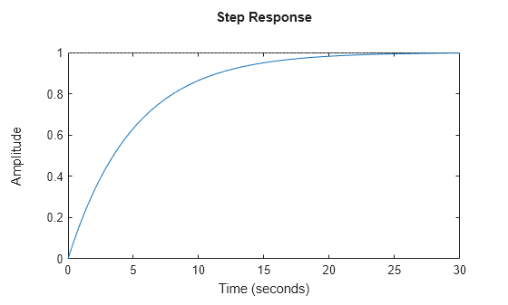
Specify reference model for tuning. The reference model describes the desired closed loop behavior of the system from reference to output.
mref = tf(1,[5 1]);
stepplot(mref)
By default, vrfttune tunes a parallel-form PI controller for the given input-output data. Tune the controller gains.
[theta,cTuned,info] = vrfttune(tt,mref)
theta = 2×1

    0.0667
   -0.0000
cTuned =

              Ts
  Kp + Ki * ------
              z-1

  with Kp = 0.0667, Ki = -1.92e-05, Ts = 0.1

Sample time: 0.1 seconds
Discrete-time PI controller in parallel form.
Model Properties
info = struct with fields:
    TuningMethod: 'least-square'
       CostValue: 5.5912
The function returns an array theta with entries corresponding to the gains Kp and Ki. The function also returns a pid object cTuned parameterized with the tuned gains and tuning information info.
Validate the closed-loop response of the original system sys with tuned controller against the reference plant mref.
cl = feedback(cTuned*sys,1);
stepplot(cl,mref,"--")
legend("Closed-loop response","Reference model")
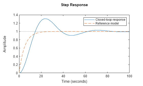
The closed-loop response does not match the desired reference. A PI controller for this plant sys does not provide enough damping and responsiveness to meet the desired reference model. Next, you can tune a PID controller and see if it provides a better match. To do so, specify additional options using vrfttuneOptions before tuning.
opt = vrfttuneOptions("parallel-pid");
opt.PIDType = "PID";
[theta2,cTuned2,info2] = vrfttune(tt,mref,VRFTOptions=opt)
theta2 = 3×1

    0.0661
    0.0000
    0.6698
cTuned2 =

              Ts               1
  Kp + Ki * ------ + Kd * -----------
              z-1         Tf+Ts/(z-1)

  with Kp = 0.0661, Ki = 2.72e-07, Kd = 0.67, Tf = 0.1, Ts = 0.1

Sample time: 0.1 seconds
Discrete-time PIDF controller in parallel form.
Model Properties
info2 = struct with fields:
    TuningMethod: 'least-square'
       CostValue: 0.0039
Compare the closed-loop response with the desired reference.
cl2 = feedback(cTuned2*sys,1);
stepplot(cl2,mref,"--")
legend("Closed-loop response","Reference model")
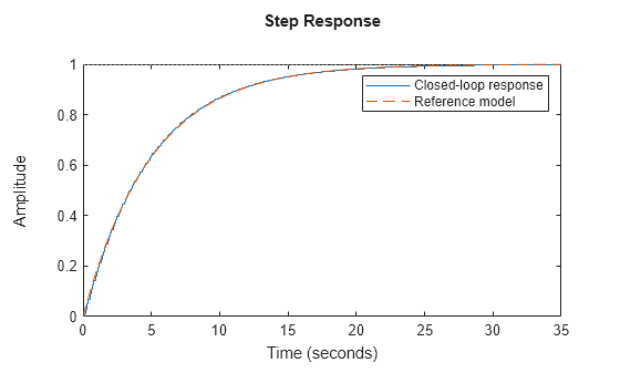
The response with tuned PID controller now closely matches the desired closed-loop reference.
This example shows how to use previously logged input-output data to tune PID controllers using the vrfttune function.
Prepare Logged Data
This example uses the input and output data logged from a Simulink® model of a mass-spring-damper plant. Load the logged data.
load TuningUsingSimulinkLoggedData.matExtract data points for the tuning interval from 1 s to 400 s. The PID controller sample time is 0.1 s.
u = tsu_simulink(11:4001);
y = tsy_simulink(11:4001);
Ts = 0.1;
t = Ts*(0:1:length(y)-1)';
To perform tuning using vrfttune, provide uniformly sampled input-output data represented by a timetable object. Create a timetable.
TT_simulink = timetable(seconds(t),u,y);
Provide Reference Model and Weight Function
Provide a reference model as an LTI object to describe the desired closed-loop performance. Optionally,provide a weighting function as an LTI object to emphasize specific frequency ranges. If you provide continuous-time LTI objects, vrfttune discretizes them before tuning. Define the reference model and weighting function.
MrefS = tf(1,[3 1]);
WeightS = tf(1,[0.3 1]);
Define Controller Structure Using Different Options
Tune PID controllers using structures supported by vrfttune. Use an option set created with vrfttuneOptions to specify the controller structure. Available options include "parallel-pid", "lti-combination", and "tunable-lti". Define the objects.
Use "parallel-pid" Option
optionsParallelPID = vrfttuneOptions('parallel-pid');
optionsParallelPID.PIDType = 'PID';
optionsParallelPID.IntegratorMethod = 'Trapezoidal';
Display the properties of the options object.
optionsParallelPID
optionsParallelPID =
  ParallelPID with properties:

                 PIDType: 'PID'
        IntegratorMethod: 'Trapezoidal'
    DiscretizationMethod: 'tustin'
Use "lti-combination" Option
optionsLTICombination = vrfttuneOptions("lti-combination");
optionsLTICombination.LinearControlBasis = {tf([1],[1],0.1); 0.1/2*tf([1 1],[1 -1],0.1); 1/0.1*tf([1 -1],[1 0],0.1)};
Display the properties of the options object.
optionsLTICombination
optionsLTICombination =
  LTICombination with properties:

      LinearControlBasis: {3×1 cell}
    DiscretizationMethod: 'tustin'
Use "tunable-lti" Option
optionsTunableLTI = vrfttuneOptions('tunable-lti');
controller = tunablePID('Ctrl','PID',0.1);
controller.IFormula = 'Trapezoidal';
controller.Kp.Free = 1;controller.Kp.Value = 0.1;controller.Kp.Minimum = 0.01;controller.Kp.Maximum = 1;
controller.Ki.Free = 1;controller.Ki.Value = 0.1;controller.Ki.Minimum = 0.01;controller.Ki.Maximum = 1;
controller.Kd.Free = 1;controller.Kd.Value = 0.1;controller.Kd.Minimum = 0.01;controller.Kd.Maximum = 1;
controller.Tf.Free = 0;controller.Tf.Value = 0.1;
optionsTunableLTI.TunableController = controller;
Define optimization options to tune controller parameters with fmincon.
optionsTunableLTI.OptimizationOptions = optimoptions('fmincon','Algorithm','sqp')
optionsTunableLTI =
  TunableLTI with properties:

       TunableController: [1×1 tunablePID]
     OptimizationOptions: [1×1 optim.options.Fmincon]
    DiscretizationMethod: 'tustin'
Tune PID Controller Parameters
Tune the PID controller parameters for the parallel PID structure.
[thetaParam_parallel_pid,tunedblk_parallel_pid,info_parallel_pid]...
    = vrfttune(TT_simulink,MrefS,WeightingFunction = WeightS,VRFTOptions=optionsParallelPID);
Tune the PID controller parameters for the LTI combination structure.
[thetaParam_lti_combination,tunedblk_lti_combination,info_lti_combination]...
    = vrfttune(TT_simulink,MrefS,WeightingFunction = WeightS,VRFTOptions=optionsLTICombination);
Tune the PID controller parameters for the tunable LTI object.
[thetaParam_tunable_lti,tunedblk_tunable_lti,info_tunable_lti]...
    = vrfttune(TT_simulink,MrefS,WeightingFunction = WeightS,VRFTOptions=optionsTunableLTI);
Local minimum found that satisfies the constraints. Optimization completed because the objective function is non-decreasing in feasible directions, to within the value of the optimality tolerance, and constraints are satisfied to within the value of the constraint tolerance. <stopping criteria details>
Compare the tuned PID parameters to the tuning result from the original Simulink model with the Virtual Reference Feedback Tuning block over the same interval.
T = table(thetaParam_simulink, thetaParam_parallel_pid, thetaParam_lti_combination, thetaParam_tunable_lti);
T.Properties.RowNames = {'Kp','Ki','Kd'}T=3×4 table
thetaParam_simulink thetaParam_parallel_pid thetaParam_lti_combination thetaParam_tunable_lti
___________________ _______________________ __________________________ ______________________
Kp 0.069745 0.069745 0.069745 0.069745
Ki 0.11114 0.11114 0.11114 0.11114
Kd 0.24576 0.24576 0.24576 0.24576
The tuning results for the PID controller using different structures are consistent.
Input Arguments
Name-Value Arguments
Output Arguments
Algorithms
For PID, FIR, and linear combination controllers, the function solves a least-squares problem to obtain the tuned parameters.
For tunable LTI models, the function uses fmincon (Optimization Toolbox) to obtain the tuned parameters. This requires Optimization Toolbox™ software.
For a summary of the VRFT algorithm, see Virtual Reference Feedback Tuning.
References
[1] Campi, M. C., A. Lecchini, and S. M. Savaresi. “Virtual Reference Feedback Tuning: A Direct Method for the Design of Feedback Controllers.” Automatica 38, no. 8 (August 1, 2002): 1337–46. https://doi.org/10.1016/S0005-1098(02)00032-8.
Version History
Introduced in R2026a