MATLAB アプリケーションの結果からのプレゼンテーションの生成

ライブスクリプトを開く

この例では、MATLAB® API for PowerPoint® (PPT API) を使用して、MATLAB アプリケーションの結果から Microsoft® PowerPoint® プレゼンテーションを生成する方法を示します。この例では、米国の人口を予測するアプリケーションの結果からプレゼンテーションを生成します。この例で生成されるスライドは次のようになります。

Five presentation slides created by the example, starting with the title slide, a slide with bullet points describing the population modeling approach, and three slides with MATLAB generated graphs.

プレゼンテーションの作成

長い完全修飾名を使用せずに済むよう、PPT 名前空間をインポートします。

import mlreportgen.ppt.*;

この例で生成されるイメージの削除を容易にするために、イメージを保持する cell 配列を作成します。

images = {};

既定のテンプレートを使用して、プレゼンテーションを作成します。

ppt = Presentation("population.pptx");
open(ppt);

プレゼンテーションへのスライドの追加

PowerPoint プレゼンテーションは、事前定義されたレイアウトから作成されるスライドで構成されています。レイアウトには、生成されたコンテンツを埋め込むプレースホルダーが含まれています。事前定義されたレイアウトは、スタイルを定義するテンプレートスライドマスターに属しています。

Title Slide レイアウトを使用して、最初のスライドをプレゼンテーションに追加します。

slide1 = add(ppt,"Title Slide");

置換メソッドを使用して、スライドのタイトルとサブタイトルを置き換えます。

replace(slide1,"Title","Modeling the US Population");
replace(slide1,"Subtitle","A Risky Business");

Title and Content レイアウトを使用して、2 番目のスライドをプレゼンテーションに追加します。タイトルを置き換えます。

slide2 = add(ppt,"Title and Content");
replace(slide2,"Title","Population Modeling Approach");

cell 配列を使用して、Content プレースホルダーにテキストを追加します。

replace(slide2,"Content",{ ...
    "Fit polynomial to US Census data", ...
    "Use polynomials to extrapolate population growth", ...
    "Based on Computer Methods for Mathematical Computations" + ...
    " by Forsythe, Malcolm and Moler," + ...
    " published by Prentice-Hall in 1977", ...
    "Varying polynomial degree shows riskiness of approach"});

Title and Content レイアウトを使用して、3 番目のスライドをプレゼンテーションに追加します。タイトルを置き換えます。

slide3 = add(ppt,"Title and Content");
replace(slide3,"Title","US Census data from 1900 to 2000");

1910 年から 2000 年までの米国国勢調査データのプロットを作成します。

% Time interval
t = (1910:10:2000)';

% Population
p = [91.972 105.711 123.203 131.669 150.697...
    179.323 203.212 226.505 249.633 281.422]';

% Plot
fig1 = figure;
plot(t,p,"bo");
axis([1910 2020 0 400]);
title("Population of the US 1910-2000");
ylabel("Millions");

プロットをイメージに変換します。プレゼンテーション生成の最後に削除するイメージのリストにイメージを追加します。プレゼンテーションを閉じるまで、イメージを削除しないでください。

img1 = "plot1.png";
saveas(fig1,img1);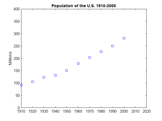

Figure contains an axes object. The axes object with title Population of the US 1910-2000, ylabel Millions contains a line object which displays its values using only markers.

images = [images {img1}];

Content プレースホルダーをイメージに置き換えます。

replace(slide3,"Content",Picture(img1));

Comparison レイアウトを使用して、4 番目のスライドをプレゼンテーションに追加します。このスライドを使用して、人口データの 3 次外挿および 4 次外挿の比較を示します。

slide4 = add(ppt,"Comparison");
replace(slide4,"Title","Polynomial Degree Changes Extrapolation");

人口データの多項式近似の係数を計算します。

n = length(t);
s = (t-1950)/50;
A = zeros(n);
A(:,end) = 1;
for j = n-1:-1:1
    A(:,j) = s .* A(:,j+1);
end
c = A(:,n-3:n)\p;

Left Text プレースホルダーをテキストに置き換えます。

replace(slide4,"Left Text","Cubic extrapolation");

3 次外挿を計算します。

v = (1910:2020)';
x = (v-1950)/50;
w = (2010-1950)/50;
y = polyval(c,x);
z = polyval(c,w);

fig2 = figure;
hold on
plot(v,y,"k-");
plot(2010,z,"ks");
text(2010,z+15,num2str(z));
hold off

プロットからイメージを作成し、削除するイメージのリストにそのイメージを追加します。

img2 = "plot2.png";
saveas(fig2,img2);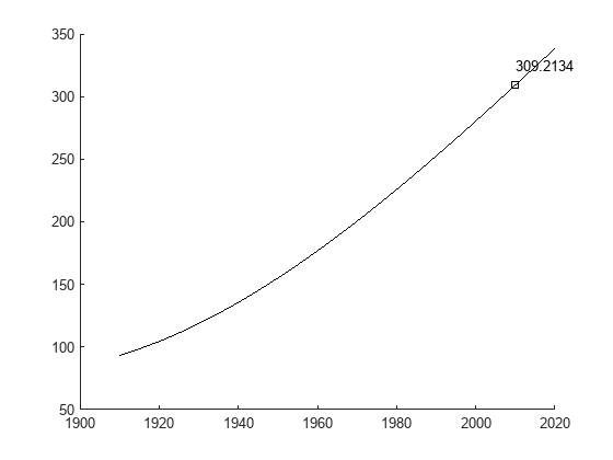

Figure contains an axes object. The axes object contains 3 objects of type line, text. One or more of the lines displays its values using only markers

images = [images {img2}];

Left Content プレースホルダーをイメージに置き換えます。

replace(slide4,"Left Content",Picture(img2));

Right Text プレースホルダーをテキストに置き換えます。

replace(slide4,"Right Text","Quartic extrapolation");

4 次外挿を計算します。

c = A(:,n-4:n)\p;
y = polyval(c,x);
z = polyval(c,w);
fig3 = figure;
hold on
plot(v,y,"k-");
plot(2010,z,"ks");
text(2010,z-15,num2str(z));
hold off

プロットからイメージを作成し、削除するイメージのリストにそのイメージを追加して、Right Content プレースホルダーをイメージに置き換えます。

img3 = "plot3.png";
saveas(fig3,img3);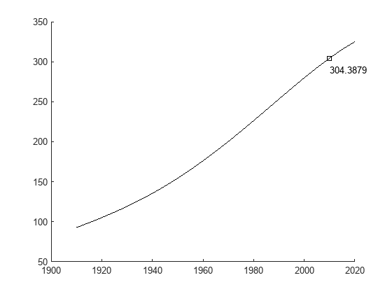

Figure contains an axes object. The axes object contains 3 objects of type line, text. One or more of the lines displays its values using only markers

images = [images {img3}];
replace(slide4,"Right Content",Picture(img3));

Title and Content レイアウトを使用して、最後のスライドをプレゼンテーションに追加します。

slide5 = add(ppt,"Title and Content");
replace(slide5,"Title",...
    "As the degree increases, the extrapolation " + ...
    "becomes even more erratic");

次数が上がると外挿がさらに不安定になることを示すプロットを作成します。

fig4 = figure;
cla
plot(t,p,"bo")
hold on
axis([1910 2020 0 400])
colors = hsv(8);
labels = {"data"};
for d = 1:8
   [Q,R] = qr(A(:,n-d:n));
   R = R(1:d+1,:);
   Q = Q(:,1:d+1);
   c = R\(Q'*p);   
   y = polyval(c,x);
   z = polyval(c,11);
   plot(v,y,"color",colors(d,:));
   labels{end+1} = "degree = " + int2str(d);
end
legend(labels, "Location", "NorthWest")
hold off

プロットからイメージを作成し、Content プレースホルダーをイメージに置き換えます。

img4 = "plot4.png";
saveas(fig4,img4);

Figure contains an axes object. The axes object contains 9 objects of type line. One or more of the lines displays its values using only markers These objects represent data, degree = 1, degree = 2, degree = 3, degree = 4, degree = 5, degree = 6, degree = 7, degree = 8.

images = [images {img4}];
replace(slide5,"Content",Picture(img4));

プレゼンテーションの終了と表示

close(ppt);
rptview(ppt);

イメージの削除

プレゼンテーションを閉じるときに、イメージがプレゼンテーションにコピーされます。これで、イメージを削除できるようになりました。

len = length(images);
for i = 1:len
    delete(images{i});
end

参考

mlreportgen.ppt.Presentation | mlreportgen.ppt.Slide

MATLAB アプリケーションの結果からのプレゼンテーションの生成

プレゼンテーションの作成

プレゼンテーションへのスライドの追加

プレゼンテーションの終了と表示

イメージの削除

参考

トピック