modelCalibrationPlot
Syntax
Description
modelCalibrationPlot(___,
specifies options using one or more name-value pair arguments in addition to the
input arguments in the previous syntax. You can use the
Name,Value)ModelLevel name-value pair argument to compute metrics
using the underlying model's transformed scale.
h = modelCalibrationPlot(ax,___,Name,Value)h.
Examples
This example shows how to use fitLGDModel to fit data with a Regression model and then use modelCalibrationPlot to generate a scatter plot for predicted and observed LGDs.
Load Data
Load the loss given default data.
load LGDData.mat
head(data)
LTV Age Type LGD
_______ _______ ___________ _________
0.89101 0.39716 residential 0.032659
0.70176 2.0939 residential 0.43564
0.72078 2.7948 residential 0.0064766
0.37013 1.237 residential 0.007947
0.36492 2.5818 residential 0
0.796 1.5957 residential 0.14572
0.60203 1.1599 residential 0.025688
0.92005 0.50253 investment 0.063182
Partition Data
Separate the data into training and test partitions.
rng('default'); % for reproducibility
NumObs = height(data);

c = cvpartition(NumObs,'HoldOut',0.4);
TrainingInd = training(c);
TestInd = test(c);
Create Regression LGD Model
Use fitLGDModel to create a Regression model using training data.
lgdModel = fitLGDModel(data(TrainingInd,:),'regression');
disp(lgdModel)
Regression with properties:
ResponseTransform: "logit"
BoundaryTolerance: 1.0000e-05
ModelID: "Regression"
Description: ""
UnderlyingModel: [1×1 classreg.regr.CompactLinearModel]
PredictorVars: ["LTV" "Age" "Type"]
ResponseVar: "LGD"
WeightsVar: ""
Display the underlying model.
lgdModel.UnderlyingModel
ans =
Compact linear regression model:
    LGD_logit ~ 1 + LTV + Age + Type

Estimated Coefficients:
                       Estimate       SE        tStat       pValue
                       ________    ________    _______    __________

    (Intercept)        -4.7549      0.36041    -13.193    3.0997e-38
    LTV                 2.8565      0.41777     6.8377    1.0531e-11
    Age                -1.5397     0.085716    -17.963    3.3172e-67
    Type_investment     1.4358       0.2475     5.8012     7.587e-09


Number of observations: 2093, Error degrees of freedom: 2089
Root Mean Squared Error: 4.24
R-squared: 0.206,  Adjusted R-Squared: 0.205
F-statistic vs. constant model: 181, p-value = 2.42e-104
Generate Scatter Plot of Predicted and Observed LGDs
Use modelCalibrationPlot to generate a scatter plot of predicted and observed LGDs for the test data set. The ModelLevel name-value argument modifies the output only for Regression models, not Tobit models, because there are no response transformations for the Tobit model.
modelCalibrationPlot(lgdModel,data(TestInd,:),ModelLevel="underlying")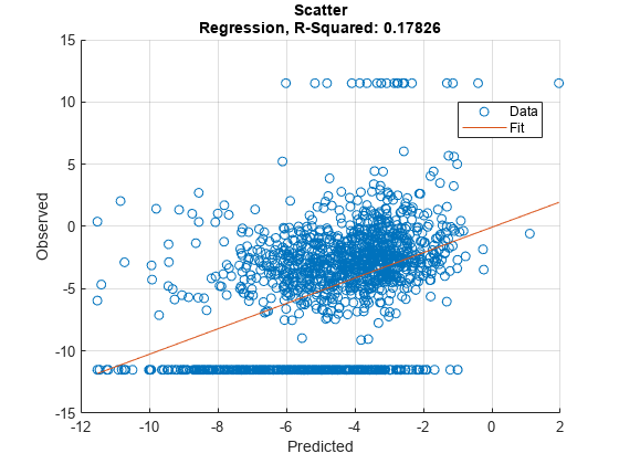
This example shows how to use fitLGDModel to fit data with a Tobit model and then use modelCalibrationPlot to generate a scatter plot of predicted and observed LGDs.
Load Data
Load the loss given default data.
load LGDData.mat
head(data)
LTV Age Type LGD
_______ _______ ___________ _________
0.89101 0.39716 residential 0.032659
0.70176 2.0939 residential 0.43564
0.72078 2.7948 residential 0.0064766
0.37013 1.237 residential 0.007947
0.36492 2.5818 residential 0
0.796 1.5957 residential 0.14572
0.60203 1.1599 residential 0.025688
0.92005 0.50253 investment 0.063182
Partition Data
Separate the data into training and test partitions.
rng('default'); % for reproducibility
NumObs = height(data);

c = cvpartition(NumObs,'HoldOut',0.4);
TrainingInd = training(c);
TestInd = test(c);
Create Tobit LGD Model
Use fitLGDModel to create a Tobit model using training data.
lgdModel = fitLGDModel(data(TrainingInd,:),'tobit');
disp(lgdModel)
Tobit with properties:
CensoringSide: "both"
LeftLimit: 0
RightLimit: 1
Weights: [0×1 double]
ModelID: "Tobit"
Description: ""
UnderlyingModel: [1×1 risk.internal.credit.TobitModel]
PredictorVars: ["LTV" "Age" "Type"]
ResponseVar: "LGD"
WeightsVar: ""
Display the underlying model.
disp(lgdModel.UnderlyingModel)
Tobit regression model:
     LGD = max(0,min(Y*,1))
     Y* ~ 1 + LTV + Age + Type

Estimated coefficients:
                       Estimate        SE         tStat       pValue
                       _________    _________    _______    __________

    (Intercept)         0.058257     0.027288     2.1349      0.032888
    LTV                  0.20126      0.03138     6.4136    1.7523e-10
    Age                -0.095407    0.0072525    -13.155             0
    Type_investment      0.10208     0.018069     5.6495    1.8283e-08
    (Sigma)              0.29288    0.0057103     51.289             0

Number of observations: 2093
Number of left-censored observations: 547
Number of uncensored observations: 1521
Number of right-censored observations: 25
Log-likelihood: -698.383
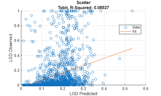
Generate Scatter Plot of Predicted and Observed LGDs
Use modelCalibrationPlot to generate a scatter plot of predicted and observed LGDs for the test data set.
modelCalibrationPlot(lgdModel,data(TestInd,:))
This example shows how to use fitLGDModel to fit data with a Beta model and then use modelCalibrationPlot to generate a scatter plot of predicted and observed LGDs.
Load Data
Load the loss given default data.
load LGDData.mat
head(data)
LTV Age Type LGD
_______ _______ ___________ _________
0.89101 0.39716 residential 0.032659
0.70176 2.0939 residential 0.43564
0.72078 2.7948 residential 0.0064766
0.37013 1.237 residential 0.007947
0.36492 2.5818 residential 0
0.796 1.5957 residential 0.14572
0.60203 1.1599 residential 0.025688
0.92005 0.50253 investment 0.063182
Partition Data
Separate the data into training and test partitions.
rng('default'); % for reproducibility
NumObs = height(data);

c = cvpartition(NumObs,'HoldOut',0.4);
TrainingInd = training(c);
TestInd = test(c);
Create Beta LGD Model
Use fitLGDModel to create a Beta model using training data.
lgdModel = fitLGDModel(data(TrainingInd,:),'Beta');
disp(lgdModel)
Beta with properties:
BoundaryTolerance: 1.0000e-05
ModelID: "Beta"
Description: ""
UnderlyingModel: [1×1 risk.internal.credit.BetaModel]
PredictorVars: ["LTV" "Age" "Type"]
ResponseVar: "LGD"
WeightsVar: ""
Display the underlying model.
disp(lgdModel.UnderlyingModel)
Beta regression model:
     logit(LGD) ~ 1_mu + LTV_mu + Age_mu + Type_mu
     log(LGD) ~ 1_phi + LTV_phi + Age_phi + Type_phi

Estimated coefficients:
                           Estimate       SE        tStat       pValue
                           ________    ________    _______    __________

    (Intercept)_mu          -1.3772     0.13201    -10.433             0
    LTV_mu                   0.6027     0.15087     3.9947    6.7017e-05
    Age_mu                 -0.47464    0.040264    -11.788             0
    Type_investment_mu      0.45372    0.085143     5.3289    1.0942e-07
    (Intercept)_phi        -0.16336     0.12591    -1.2974       0.19463
    LTV_phi                0.055886     0.14719    0.37968       0.70422
    Age_phi                 0.22887    0.040335     5.6743    1.5865e-08
    Type_investment_phi    -0.14102    0.078155    -1.8044      0.071313

Number of observations: 2093
Log-likelihood: -5291.04
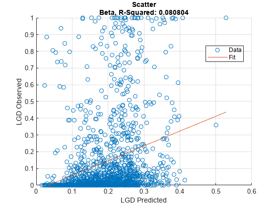
Generate Scatter Plot of Predicted and Observed LGDs
Use modelCalibrationPlot to generate a scatter plot of predicted and observed LGDs for the test data set.
modelCalibrationPlot(lgdModel,data(TestInd,:))
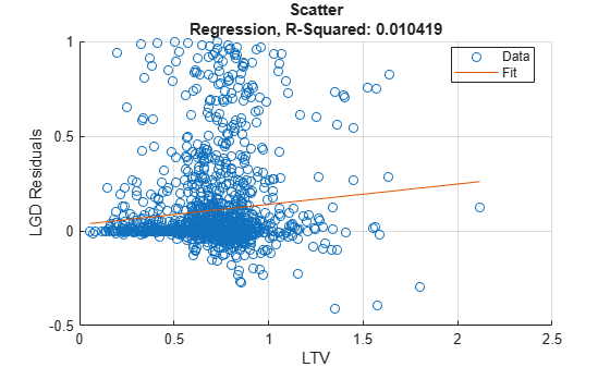
modelCalibrationPlot generates a scatter plot of observed vs. predicted LGD values. The 'XData' and 'YData' name-value arguments allow you to visualize the residuals or generate a scatter plot against a variable of interest.
Load Data
Load the loss given default data.
load LGDData.mat
head(data)
LTV Age Type LGD
_______ _______ ___________ _________
0.89101 0.39716 residential 0.032659
0.70176 2.0939 residential 0.43564
0.72078 2.7948 residential 0.0064766
0.37013 1.237 residential 0.007947
0.36492 2.5818 residential 0
0.796 1.5957 residential 0.14572
0.60203 1.1599 residential 0.025688
0.92005 0.50253 investment 0.063182
Partition Data
Separate the data into training and test partitions.
rng('default'); % for reproducibility
NumObs = height(data);

c = cvpartition(NumObs,'HoldOut',0.4);
TrainingInd = training(c);
TestInd = test(c);
Create Regression LGD Model
Use fitLGDModel to create a Regression model using training data.
lgdModel = fitLGDModel(data(TrainingInd,:),'regression');
disp(lgdModel)
Regression with properties:
ResponseTransform: "logit"
BoundaryTolerance: 1.0000e-05
ModelID: "Regression"
Description: ""
UnderlyingModel: [1×1 classreg.regr.CompactLinearModel]
PredictorVars: ["LTV" "Age" "Type"]
ResponseVar: "LGD"
WeightsVar: ""
Display the underlying model.
disp(lgdModel.UnderlyingModel)
Compact linear regression model:
    LGD_logit ~ 1 + LTV + Age + Type

Estimated Coefficients:
                       Estimate       SE        tStat       pValue
                       ________    ________    _______    __________

    (Intercept)        -4.7549      0.36041    -13.193    3.0997e-38
    LTV                 2.8565      0.41777     6.8377    1.0531e-11
    Age                -1.5397     0.085716    -17.963    3.3172e-67
    Type_investment     1.4358       0.2475     5.8012     7.587e-09


Number of observations: 2093, Error degrees of freedom: 2089
Root Mean Squared Error: 4.24
R-squared: 0.206,  Adjusted R-Squared: 0.205
F-statistic vs. constant model: 181, p-value = 2.42e-104
Generate Scatter Plot of Predicted and Observed LGDs
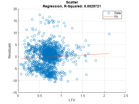
Use modelCalibrationPlot to generate a scatter plot of residuals against LTV values.
modelCalibrationPlot(lgdModel,data(TestInd,:),XData='LTV',YData='residuals')
For Regression models, the 'ModelLevel' name-value argument allows you to visualize the plot using the underlying model scale.
modelCalibrationPlot(lgdModel,data(TestInd,:),XData='LTV',YData='residuals',ModelLevel='underlying')
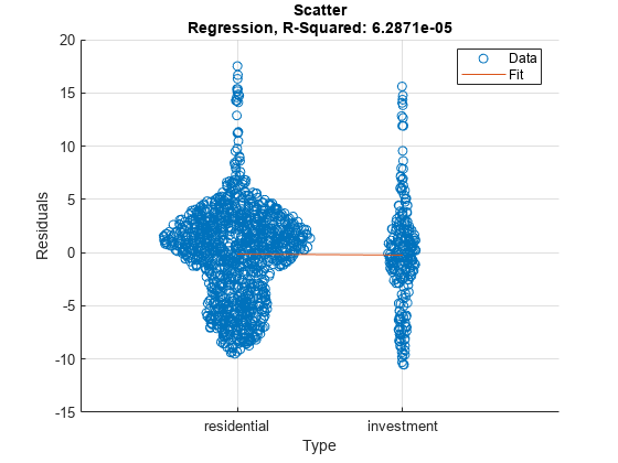
For categorical variables, modelCalibrationPlot uses a swarm chart. For more information, see swarmchart.
modelCalibrationPlot(lgdModel,data(TestInd,:),XData='Type',YData='residuals',ModelLevel='underlying')
Input Arguments
Name-Value Arguments
Output Arguments
More About
References
[1] Baesens, Bart, Daniel Roesch, and Harald Scheule. Credit Risk Analytics: Measurement Techniques, Applications, and Examples in SAS. Wiley, 2016.
[2] Bellini, Tiziano. IFRS 9 and CECL Credit Risk Modelling and Validation: A Practical Guide with Examples Worked in R and SAS. San Diego, CA: Elsevier, 2019.
Version History
Introduced in R2023a
See Also
Tobit | Regression | Beta | modelCalibration | modelDiscriminationPlot | modelDiscrimination | predict | fitLGDModel