modelDiscriminationPlot
Plot ROC curve
Syntax
Description
modelDiscriminationPlot(___,
specifies options using one or more name-value pair arguments in addition to the
input arguments in the previous syntax.Name,Value)
h = modelDiscriminationPlot(ax,___,Name,Value)h.
Examples
This example shows how to use fitLGDModel to fit data with a Regression model and then use modelDiscriminationPlot to plot the ROC.
Load Data
Load the loss given default data.
load LGDData.mat
head(data)
LTV Age Type LGD
_______ _______ ___________ _________
0.89101 0.39716 residential 0.032659
0.70176 2.0939 residential 0.43564
0.72078 2.7948 residential 0.0064766
0.37013 1.237 residential 0.007947
0.36492 2.5818 residential 0
0.796 1.5957 residential 0.14572
0.60203 1.1599 residential 0.025688
0.92005 0.50253 investment 0.063182
Partition Data
Separate the data into training and test partitions.
rng('default'); % for reproducibility
NumObs = height(data);

c = cvpartition(NumObs,'HoldOut',0.4);
TrainingInd = training(c);
TestInd = test(c);
Create a Regression LGD Model
Use fitLGDModel to create a Regression model using training data.
lgdModel = fitLGDModel(data(TrainingInd,:),'regression');
disp(lgdModel)
Regression with properties:
ResponseTransform: "logit"
BoundaryTolerance: 1.0000e-05
ModelID: "Regression"
Description: ""
UnderlyingModel: [1×1 classreg.regr.CompactLinearModel]
PredictorVars: ["LTV" "Age" "Type"]
ResponseVar: "LGD"
WeightsVar: ""
Display the underlying model.
disp(lgdModel.UnderlyingModel)
Compact linear regression model:
    LGD_logit ~ 1 + LTV + Age + Type

Estimated Coefficients:
                       Estimate       SE        tStat       pValue
                       ________    ________    _______    __________

    (Intercept)        -4.7549      0.36041    -13.193    3.0997e-38
    LTV                 2.8565      0.41777     6.8377    1.0531e-11
    Age                -1.5397     0.085716    -17.963    3.3172e-67
    Type_investment     1.4358       0.2475     5.8012     7.587e-09


Number of observations: 2093, Error degrees of freedom: 2089
Root Mean Squared Error: 4.24
R-squared: 0.206,  Adjusted R-Squared: 0.205
F-statistic vs. constant model: 181, p-value = 2.42e-104
Plot ROC Data
Use modelDiscriminationPlot to plot the ROC for the test data set.
modelDiscriminationPlot(lgdModel,data(TestInd,:))

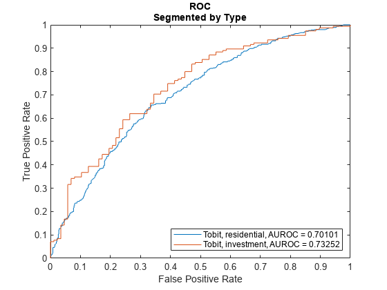
This example shows how to use fitLGDModel to fit data with a Tobit model and then use modelDiscriminationPlot to plot the ROC.
Load Data
Load the loss given default data.
load LGDData.mat
head(data)
LTV Age Type LGD
_______ _______ ___________ _________
0.89101 0.39716 residential 0.032659
0.70176 2.0939 residential 0.43564
0.72078 2.7948 residential 0.0064766
0.37013 1.237 residential 0.007947
0.36492 2.5818 residential 0
0.796 1.5957 residential 0.14572
0.60203 1.1599 residential 0.025688
0.92005 0.50253 investment 0.063182
Partition Data
Separate the data into training and test partitions.
rng('default'); % for reproducibility
NumObs = height(data);

c = cvpartition(NumObs,'HoldOut',0.4);
TrainingInd = training(c);
TestInd = test(c);
Create a Tobit LGD Model
Use fitLGDModel to create a Tobit model using training data.
lgdModel = fitLGDModel(data(TrainingInd,:),'tobit');
disp(lgdModel)
Tobit with properties:
CensoringSide: "both"
LeftLimit: 0
RightLimit: 1
Weights: [0×1 double]
ModelID: "Tobit"
Description: ""
UnderlyingModel: [1×1 risk.internal.credit.TobitModel]
PredictorVars: ["LTV" "Age" "Type"]
ResponseVar: "LGD"
WeightsVar: ""
Display the underlying model.
disp(lgdModel.UnderlyingModel)
Tobit regression model:
     LGD = max(0,min(Y*,1))
     Y* ~ 1 + LTV + Age + Type

Estimated coefficients:
                       Estimate        SE         tStat       pValue
                       _________    _________    _______    __________

    (Intercept)         0.058257     0.027288     2.1349      0.032888
    LTV                  0.20126      0.03138     6.4136    1.7523e-10
    Age                -0.095407    0.0072525    -13.155             0
    Type_investment      0.10208     0.018069     5.6495    1.8283e-08
    (Sigma)              0.29288    0.0057103     51.289             0

Number of observations: 2093
Number of left-censored observations: 547
Number of uncensored observations: 1521
Number of right-censored observations: 25
Log-likelihood: -698.383
Plot ROC Data
Use modelDiscriminationPlot to plot the ROC for the test data set.
modelDiscriminationPlot(lgdModel,data(TestInd,:),"SegmentBy","Type","DiscretizeBy","median")

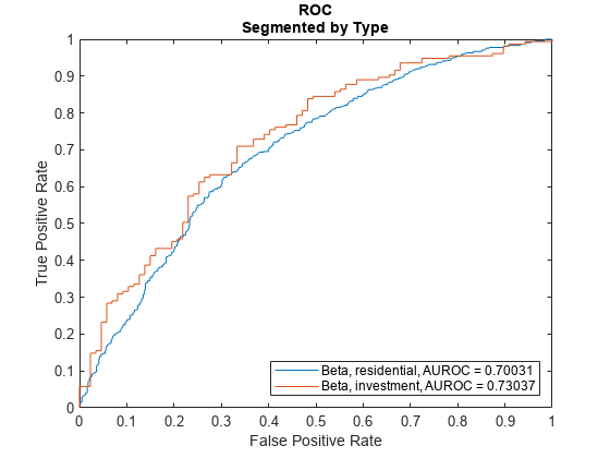
This example shows how to use fitLGDModel to fit data with a Beta model and then use modelDiscriminationPlot to plot the ROC.
Load Data
Load the loss given default data.
load LGDData.mat
head(data)
LTV Age Type LGD
_______ _______ ___________ _________
0.89101 0.39716 residential 0.032659
0.70176 2.0939 residential 0.43564
0.72078 2.7948 residential 0.0064766
0.37013 1.237 residential 0.007947
0.36492 2.5818 residential 0
0.796 1.5957 residential 0.14572
0.60203 1.1599 residential 0.025688
0.92005 0.50253 investment 0.063182
Partition Data
Separate the data into training and test partitions.
rng('default'); % for reproducibility
NumObs = height(data);

c = cvpartition(NumObs,'HoldOut',0.4);
TrainingInd = training(c);
TestInd = test(c);
Create a Beta LGD Model
Use fitLGDModel to create a Beta model using training data.
lgdModel = fitLGDModel(data(TrainingInd,:),'Beta');
disp(lgdModel)
Beta with properties:
BoundaryTolerance: 1.0000e-05
ModelID: "Beta"
Description: ""
UnderlyingModel: [1×1 risk.internal.credit.BetaModel]
PredictorVars: ["LTV" "Age" "Type"]
ResponseVar: "LGD"
WeightsVar: ""
Display the underlying model.
disp(lgdModel.UnderlyingModel)
Beta regression model:
     logit(LGD) ~ 1_mu + LTV_mu + Age_mu + Type_mu
     log(LGD) ~ 1_phi + LTV_phi + Age_phi + Type_phi

Estimated coefficients:
                           Estimate       SE        tStat       pValue
                           ________    ________    _______    __________

    (Intercept)_mu          -1.3772     0.13201    -10.433             0
    LTV_mu                   0.6027     0.15087     3.9947    6.7017e-05
    Age_mu                 -0.47464    0.040264    -11.788             0
    Type_investment_mu      0.45372    0.085143     5.3289    1.0942e-07
    (Intercept)_phi        -0.16336     0.12591    -1.2974       0.19463
    LTV_phi                0.055886     0.14719    0.37968       0.70422
    Age_phi                 0.22887    0.040335     5.6743    1.5865e-08
    Type_investment_phi    -0.14102    0.078155    -1.8044      0.071313

Number of observations: 2093
Log-likelihood: -5291.04
Plot ROC Data
Use modelDiscriminationPlot to plot the ROC for the test data set.
modelDiscriminationPlot(lgdModel,data(TestInd,:),"SegmentBy","Type","DiscretizeBy","median")

Input Arguments
Loss given default model, specified as a previously created Regression,
Tobit, or Beta object using
fitLGDModel.
Data Types: object
Data, specified as a
NumRows-by-NumCols table with
predictor and response values. The variable names and data types must be
consistent with the underlying model.
Data Types: table
(Optional) Valid axis object, specified as an ax object
that is created using axes. The plot will be
created in the axes specified by the optional ax argument
instead of in the current axes (gca). The optional argument
ax must precede any of the input argument
combinations.
Data Types: object
Name-Value Arguments
Specify optional pairs of arguments as
Name1=Value1,...,NameN=ValueN, where Name is
the argument name and Value is the corresponding value.
Name-value arguments must appear after other arguments, but the order of the
pairs does not matter.
Before R2021a, use commas to separate each name and value, and enclose
Name in quotes.
Example: modelDiscriminationPlot(lgdModel,data(TestInd,:),'DataID','Testing','DiscretizeBy','median')
Data set identifier, specified as the comma-separated pair consisting
of 'DataID' and a character vector or string. The
DataID is included in the output for reporting
purposes.
Data Types: char | string
Discretization method for LGD data, specified as
the comma-separated pair consisting of 'DiscretizeBy'
and a character vector or string.
'mean'— Discretized response is1if observed LGD is greater than or equal to the mean LGD,0otherwise.'median'— Discretized response is1if observed LGD is greater than or equal to the median LGD,0otherwise.'positive'— Discretized response is1if observed LGD is positive,0otherwise (full recovery).'total'— Discretized response is1if observed LGD is greater than or equal to1(total loss),0otherwise.
Data Types: char | string
Name of a column in the data input, not
necessarily a model variable, to be used to segment the data set,
specified as the comma-separated pair consisting of
'SegmentBy' and a character vector or string. One
AUROC is reported for each segment, and the corresponding ROC data for
each segment is returned in the optional output.
Data Types: char | string
Identifier for the reference model, specified as the comma-separated
pair consisting of 'ReferenceID' and a character
vector or string. 'ReferenceID' is used in the plot
for reporting purposes.
Data Types: char | string
Output Arguments
Figure handle for the line objects, returned as handle object.
More About
The modelDiscriminationPlot function plots the
receiver operator characteristic (ROC) curve.
The modelDiscriminationPlot function also shows the area under
the receiver operator characteristic (AUROC) curve, sometimes called simply the area
under the curve (AUC). This metric is between 0 and 1 and higher values indicate
better discrimination.
A numeric prediction and a binary response are needed to plot the ROC and compute
the AUROC. For LGD models, the predicted LGD is used directly as the prediction.
However, the observed LGD must be discretized into a binary variable. By default,
observed LGD values greater than or equal to the mean observed LGD are assigned a
value of 1, and values below the mean are assigned a value of 0. This discretized
response is interpreted as "high LGD" vs. "low LGD." The ROC curve and the AUROC
curve measure how well the predicted LGD separates the "high LGD" vs. the "low LGD"
observations. The discretization criterion can be changed with the
DiscretizeBy name-value pair argument for
modelDiscriminationPlot.
The ROC curve is a parametric curve that plots the proportion of
High LGD cases with predicted LGD greater than or equal to a parameter t, or true positive rate (TPR)
Low LGD cases with predicted LGD greater than or equal to the same parameter t, or false positive rate (FPR)
The parameter t sweeps through all the observed predicted LGD
values for the given data. If the AUROC value or the ROC curve data are needed
programmatically, use the modelDiscrimination function. For more information about ROC curves,
see ROC Curve and Performance Metrics.
References
[1] Baesens, Bart, Daniel Roesch, and Harald Scheule. Credit Risk Analytics: Measurement Techniques, Applications, and Examples in SAS. Wiley, 2016.
[2] Bellini, Tiziano. IFRS 9 and CECL Credit Risk Modelling and Validation: A Practical Guide with Examples Worked in R and SAS. San Diego, CA: Elsevier, 2019.
Version History
Introduced in R2021aThe lgdModel input supports an option for a
Beta model object that you can create using fitLGDModel.
The Regression and Tobit LGD models support a
reference LGD outside of the [0,1] range.
See Also
Tobit | Regression | modelCalibration | modelCalibrationPlot | modelDiscrimination | predict | fitLGDModel
MATLAB Command
You clicked a link that corresponds to this MATLAB command:
Run the command by entering it in the MATLAB Command Window. Web browsers do not support MATLAB commands.
Web サイトの選択
Web サイトを選択すると、翻訳されたコンテンツにアクセスし、地域のイベントやサービスを確認できます。現在の位置情報に基づき、次のサイトの選択を推奨します:
また、以下のリストから Web サイトを選択することもできます。
最適なサイトパフォーマンスの取得方法
中国のサイト (中国語または英語) を選択することで、最適なサイトパフォーマンスが得られます。その他の国の MathWorks のサイトは、お客様の地域からのアクセスが最適化されていません。
南北アメリカ
- América Latina (Español)
- Canada (English)
- United States (English)
ヨーロッパ
- Belgium (English)
- Denmark (English)
- Deutschland (Deutsch)
- España (Español)
- Finland (English)
- France (Français)
- Ireland (English)
- Italia (Italiano)
- Luxembourg (English)
- Netherlands (English)
- Norway (English)
- Österreich (Deutsch)
- Portugal (English)
- Sweden (English)
- Switzerland
- United Kingdom (English)