Load Predefined Control System Environments

Reinforcement Learning Toolbox™ software provides several predefined environments representing dynamical systems that are often used as benchmark cases for control systems design.

You can use predefined control system environments to learn how to apply reinforcement learning to the control of physical systems, gain familiarity with Reinforcement Learning Toolbox software features, or test your own agents. You can also use the predefined control system environments as a starting point for developing your own control system environment.

To create your own custom environments instead, see Custom Environments.

In the predefined control system environments, the state and observation are predefined and belong to nonfinite numerical vector spaces, while the action, also predefined, can still belong to a finite set. The (deterministic) state transitions laws are derived by discretizing the dynamics of an underlying physical system.

Simulink^® environments are environments that rely on an underlying model for the calculation of the state transition, reward, and observation. These environments do not support using reset and step functions. Some of the predefined control system environments are Simulink environments.

By contrast, environments that instead rely on MATLAB^® functions or objects for the calculation of the state transition, reward, and observation, are referred to as MATLAB environments.

Multiagent environments are environments in which you can train and simulate multiple agents together. Some of the predefined MATLAB and Simulink control system environments are multiagent environments. For more information on predefined multiagent environments, see Load Predefined Multiagent Environments.

To load the predefined MATLAB control system environments listed in this table, use the rlPredefinedEnv function. Each predefined environment is available in two versions, one with a discrete action space, and the other with a continuous action space.

Environment	Agent Task
Double integrator	Control a second-order dynamic system using either a discrete or continuous action space.
Cart-pole	Balance a pole on a moving cart by applying forces to the cart using either a discrete or continuous action space.
Simple pendulum with image observation	Swing up and balance a simple pendulum using the pendulum image as an observation, with either a discrete or continuous action space.

You can also load the following predefined Simulink environments using the rlPredefinedEnv function. For these environments, rlPredefinedEnv creates a SimulinkEnvWithAgent object. Each of these predefined environment is also available in two versions, one with a discrete action space, and the other with a continuous action space.

Environment	Agent Task
Simple pendulum Simulink model	Swing up and balance a simple pendulum by applying a torque to the pendulum, using either a discrete or continuous action space.
Cart-pole Simscape™ model	Balance a pole on a moving cart by applying forces to the cart using either a discrete or continuous action space. This environment relies on a Simulink model that uses Simscape blocks to model the system.

You can also load predefined grid world environments. For more information, see Load Predefined Grid World Environments.

To learn how to create your own custom environment, see Create Custom Environment Using Step and Reset Functions, Create Custom Simulink Environments, and Create Custom Environment from Class Template.

MATLAB Double-Integrator Environment

The double-integrator environment is a predefined MATLAB environment in which the goal of the agent is to control the position (right-positive) of a mass in a frictionless mono-dimensional space by applying a force input. The system has a second-order dynamics that can be represented by a double integrator, that is, two integrators in series.

In this environment, a training or simulation episode ends when either of these events occurs:

• The mass moves beyond a given threshold (by default, 5 meters) from the origin.

• The norm of the state vector is less than a given threshold (by default, 0.01).

There are two double-integrator environment variants, which differ by the agent action space:

• Discrete — The agent can apply a force of either F_max, zero, or -F_max to the cart, where F_max is the MaxForce property of the environment.

• Continuous — The agent can apply any force within the range [-F_max,F_max].

To create a double-integrator environment, use rlPredefinedEnv as follows, depending on the action space:

• Discrete action space:

  env = rlPredefinedEnv("DoubleIntegrator-Discrete");

  env = 
  
    DoubleIntegratorDiscreteAction with properties:
  
               Gain: 1
                 Ts: 0.1000
        MaxDistance: 5
      GoalThreshold: 0.0100
                  Q: [2×2 double]
                  R: 0.0100
           MaxForce: 2
              State: [2×1 double]

  For an example showing how to train an agent to control a discrete double-integrator environment, see Train PG Agent with Custom Networks to Control Discrete Double Integrator. For an example comparing the most used discrete action space agents on this environment, see Compare Agents on the Discrete Double-Integrator Environment.

• Continuous action space:

  env = rlPredefinedEnv("DoubleIntegrator-Continuous")

  env = 
  
    DoubleIntegratorContinuousAction with properties:
  
               Gain: 1
                 Ts: 0.1000
        MaxDistance: 5
      GoalThreshold: 0.0100
                  Q: [2×2 double]
                  R: 0.0100
           MaxForce: Inf
              State: [2×1 double]

  For an example showing how to train an agent to control a continuous double-integrator environment, see Compare DDPG Agent to LQR Controller. For an example comparing the most used continuous action space agents on this environment, see Compare Agents on the Continuous Double Integrator Environment.

Environment Visualization

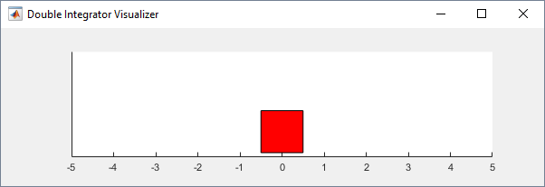
You can visualize the double-integrator environment using the plot function. The plot displays the mass as a red rectangle.

plot(env)

To visualize the environment during training, call plot before training and keep the visualization figure open.

Note

While visualizing the environment during training might often be insightful, doing so tends to increase training time. For faster training, keep the environment plot closed during training.

Environment Properties

All the environment properties listed in this table are writable. You can change them to customize the double-integrator environment to your needs.

Property	Description	Default
Gain	Gain for the double integrator. This gain multiplies the force applied to the mass.	1
Ts	Sample time in seconds. The software uses the sample time to discretize the dynamics of the underlying continuous-time system. The discrete-time dynamics is then used to calculate the next state as a function of the current state and of the applied action.	0.1
MaxDistance	Distance magnitude threshold in meters. The episode terminates if the distance is greater than this threshold.	5
GoalThreshold	State norm threshold. The episode terminates if the state is greater than this threshold.	0.01
Q	Weight matrix for the observation component of the reward signal	[10 0; 0 1]
R	Weight matrix for the action component of the reward signal	0.01
MaxForce	Maximum input force in newtons. If the magnitude of the input force exceeds this threshold, the magnitude of the force that is actually applied to the mass is limited to MaxForce.	Discrete: 2 Continuous: Inf
State	Environment state, specified as a column vector with the following state variables: Mass position Time derivative of mass position	[0 0]'

Dynamics

The continuous-time dynamics of this environment are described by this equation.

$$\ddot{p}(t)=kF(t)$$

Here, p is the position of the mass, F is the force applied by the agent, and k is the value of the Gain property. The discrete-time dynamics is then obtained using the zero-order hold approximation with sample time Ts. For more information on the used discretization method, see lqrd (Control System Toolbox).

Actions

The agent interacts with the environment using an action channel carrying a single scalar, the force applied to the mass. The action space specification is as follows:

• For the environment with discrete action space, the action channel specification is an rlFiniteSetSpec object.

  actInfo = getActionInfo(env)

  actInfo = 
  
    rlFiniteSetSpec with properties:
  
         Elements: [-2 0 2]
             Name: "force"
      Description: [0×0 string]
        Dimension: [1 1]
         DataType: "double"

• For the environment with a continuous action space, the action channel specification is an rlNumericSpec object.

  actInfo = getActionInfo(env)

  actInfo = 
  
    rlNumericSpec with properties:
  
       LowerLimit: -Inf
       UpperLimit: Inf
             Name: "force"
      Description: [0×0 string]
        Dimension: [1 1]
         DataType: "double"

For more information on obtaining action specifications from an environment, see getActionInfo.

Observations

In the double-integrator system, the agent can observe both of the environment state variables stored in env.State. The observation has a single channel, specified by an rlNumericSpec object, because both states are continuous.

obsInfo = getObservationInfo(env)

obsInfo = 

  rlNumericSpec with properties:

     LowerLimit: -Inf
     UpperLimit: Inf
           Name: "states"
    Description: "x, dx"
      Dimension: [2 1]
       DataType: "double"

For more information on obtaining observation specifications from an environment, see getObservationInfo.

Rewards

The reward signal ${\mathit{r}}_{\mathit{t+1}}$, provided at every time step, is a discretization of $\mathit{r}\left(\mathit{t}\right)$:

$$\mathit{r}\left(\mathit{t}\right)=-\left({\mathit{x}\left(\mathit{t}\right)}^{\prime }\mathit{Q}\mathit{x}\left(\mathit{t}\right)+{\mathit{u}\left(\mathit{t}\right)}^{\prime }\mathit{R}\mathit{u}\left(\mathit{t}\right)\right),$$

where:

• $\mathit{x}$ is the state vector of the system.

• $\mathit{u}$ is the force applied to the mass.

• $\mathit{Q}$ is the weight matrix on the control performance, with default value $\mathit{Q}=\left[100;01\right]$.

• $\mathit{R}$ is the weight matrix on the control effort, with default value $\mathit{R}=0.01$.

In some control system applications, the reward signal ${\mathit{r}}_{\mathit{k}}$ is also referred to as the negative of the cost at stage k.

Note that $\mathit{r}\left(\mathit{t}\right)$ is the instantaneous equivalent of this cumulative continuous-time reward, which is analogous to the cost function of an LQR controller:

$$reward=-{\displaystyle \int \left(x\text{'}Qx+u\text{'}Ru\right)}dt$$

For more information on the discretization of an LQR cost function, see lqrd (Control System Toolbox).

Reset Function

The reset function randomly sets the initial state of the environment so that the mass is still and situated at 80% of MaxDistance in either the positive or negative direction.

x0 = reset(env)

x0 =

     4
     0

Unlike other environments, you cannot set your own reset function for a double-integrator environment.

Create a Default Agent for this Environment

The environment observation and action specifications allow you to create an agent that works with your environment. For example, for the discrete action space version of this environment, create a default PG agent.

pgAgent = rlPGAgent(obsInfo,actInfo)

pgAgent = 

  rlPGAgent with properties:

            AgentOptions: [1×1 rl.option.rlPGAgentOptions]
    UseExplorationPolicy: 1
         ObservationInfo: [1×1 rl.util.rlNumericSpec]
              ActionInfo: [1×1 rl.util.rlFiniteSetSpec]
              SampleTime: 1

If needed, modify the agent options using dot notation.

pgAgent.AgentOptions.CriticOptimizerOptions.LearnRate = 1e-3;
pgAgent.AgentOptions.ActorOptimizerOptions.LearnRate = 1e-3;

You can now use both the environment and the agent as arguments for the built-in functions train and sim, which train or simulate the agent within the environment, respectively.

You can also create and train agents for this environment interactively using the Reinforcement Learning Designer app. For an example, see Design and Train Agent Using Reinforcement Learning Designer.

For more information on creating agents, see Reinforcement Learning Agents.

Step Function

You can also call the environment step function to return the next observation, reward, and an is-done scalar indicating whether a final state has been reached.

For example, call the step function with an input force of -10 N.

[xn,rn,id] = step(env,-10)

xn =

    3.9500
   -1.0000


rn =

  -16.0005


id =

  logical

   0

The environment step and reset functions allow you to create a custom training or simulation loop. For more information on custom training loops, see Train Reinforcement Learning Policy Using Custom Training Loop.

Environment Code

To access the functions that returns the discrete action space version of this environment, at the MATLAB command line, type:

edit rl.env.DoubleIntegratorDiscreteAction

To access the function that returns the continuous action space version of this environment, at the MATLAB command line, type:

edit rl.env.DoubleIntegratorContinuousAction

To access the abstract class that contains the step function, at the MATLAB command line, type:

edit rl.env.DoubleIntegratorAbstract

MATLAB Cart-Pole Environment

A MATLAB cart-pole environment is a predefined environment in which the goal of the agent is to balance a pole on a moving cart by applying a horizontal force to the cart. The pole is considered successfully balanced if both of these conditions are satisfied at the same time:

• The pole angle (clockwise positive) remains within a given threshold of the vertical position, where the vertical position is zero radians.

• The magnitude of the cart position (right positive) remains below a given threshold.

In this environment, a training or simulation episode ends when either of these events occurs:

• The magnitude of the pole angle with respect to the vertical axis is more than a given threshold (by default, 12 degrees).

• The cart moves more than a predefined threshold (by default, 2.4 meters) from the original position.

There are two cart-pole environment variants, which differ by the agent action space:

• Discrete — The agent can apply a force of either F_max or -F_max to the cart, where F_max is the MaxForce property of the environment (by default, 10 newtons).

• Continuous — The agent can apply any force within the range [-F_max,F_max].

To create a cart-pole environment, use rlPredefinedEnv as follows, depending on the desired action space:

• Discrete action space:

  env = rlPredefinedEnv("CartPole-Discrete")

    CartPoleDiscreteAction with properties:
  
                    Gravity: 9.8000
                   MassCart: 1
                   MassPole: 0.1000
                     Length: 0.5000
                   MaxForce: 10
                         Ts: 0.0200
      ThetaThresholdRadians: 0.2094
                 XThreshold: 2.4000
        RewardForNotFalling: 1
          PenaltyForFalling: -5
                      State: [4×1 double]
  

  For examples showing how to train an agent in this environments, see Train DQN Agent to Balance Discrete Cart-Pole System and Train PG Agent to Balance Discrete Cart-Pole System. For an example comparing the most used discrete action space agents on this environment, see Compare Agents on the Discrete Cart-Pole Environment.

• Continuous action space:

  env = rlPredefinedEnv("CartPole-Continuous")

    CartPoleContinuousAction with properties:
  
                    Gravity: 9.8000
                   MassCart: 1
                   MassPole: 0.1000
                     Length: 0.5000
                   MaxForce: 10
                         Ts: 0.0200
      ThetaThresholdRadians: 0.2094
                 XThreshold: 2.4000
        RewardForNotFalling: 1
          PenaltyForFalling: -50
                      State: [4×1 double]
  

  For an example showing how to train an agent in this environments, see Train MBPO Agent to Balance Continuous Cart-Pole System. For an example comparing the most used continuous action space agents on this environment, see Compare Agents on the Continuous Cart Pole.

Environment Properties

All the environment properties listed below are writable. You can change them to customize the cart-pole environment to your needs.

Property	Description	Default
Gravity	Acceleration due to gravity in meters per second squared	9.8
MassCart	Mass of the cart in kilograms	1
MassPole	Mass of the pole in kilograms	0.1
Length	Distance from the pole hinge to the cart center of mass. If the pole density is uniform, this is half the length of the pole.	0.5
MaxForce	Maximum horizontal force magnitude in newtons. If the magnitude of the input force exceeds this threshold, the magnitude of the force that is actually applied to the cart is limited to MaxForce.	10
Ts	Sample time in seconds. The software uses the sample time to discretize the dynamics of the underlying continuous-time system. The discrete-time dynamics is then used to calculate the next state as a function of the current state and of the applied action.	0.02
ThetaThresholdRadians	Pole angle threshold in radians. The episode terminates if the pole angle is greater than this threshold.	0.2094
XThreshold	Cart position threshold in meters. The episode terminates if the cart position is greater than this threshold.	2.4
RewardForNotFalling	Reward for each time step the pole is balanced	1
PenaltyForFalling	Reward penalty for failing to balance the pole	Discrete — -5 Continuous — -50
State	Environment state, specified as a column vector with these state variables: Cart position (right-positive, meters) Derivative of cart position (meters per second) Pole angle (clockwise-positive, radians) Derivative of pole angle (radians per second)	[0 0 0 0]'

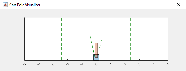
Visualization

You can visualize the cart-pole environment using the plot function. The plot displays the cart as a blue square and the pole as a red rectangle.

plot(env)

To visualize the environment during training, call plot before training and keep the visualization figure open.

Note

While visualizing the environment during training might often be insightful, doing so tends to increase training time. For faster training, keep the environment plot closed during training.

Dynamics

The cart is subjected to an external input force and can move horizontally (the horizontal axis points right). Neither the cart nor the pole is subject to friction. The pole can rotate about the hinge on the upper surface of the cart (clockwise rotations are positive). Gravity acts vertically downwards. The center of gravity of the cart is at its geometrical center, and the center of gravity of the pole is at its half length. The continuous-time equations used to model this system are described in the Examples of Cart-Pole System in Reinforcement Learning Toolbox section of the example Derive Equations of Motion and Simulate Cart-Pole System (Symbolic Math Toolbox) and the reference [2] therein. The discrete-time dynamics of the environment are then obtained using the Euler integration method.

Actions

The agent interacts with the environment using an action channel carrying a single scalar, the horizontal force applied to the cart. The action space specification is as follows:

• For an environment with a discrete action space, the action channel is specification is an rlFiniteSetSpec object.

  actInfo = getActionInfo(env)

    rlFiniteSetSpec with properties:
  
         Elements: [-10 10]
             Name: "CartPole Action"
      Description: [0×0 string]
        Dimension: [1 1]
         DataType: "double"

• For an environment with a continuous action space, the action specification is an rlNumericSpec object.

  actInfo = getActionInfo(env)

    rlNumericSpec with properties:
  
       LowerLimit: -10
       UpperLimit: 10
             Name: "CartPole Action"
      Description: [0×0 string]
        Dimension: [1 1]
         DataType: "double"

For more information on obtaining action specifications from an environment, see getActionInfo.

Observations

In the cart-pole system, the agent can observe all the environment state variables stored in env.State. The observation has a single channel specified by an rlNumericSpec object, because both signals are continuous.

obsInfo = getObservationInfo(env)

obsInfo = 

  rlNumericSpec with properties:

     LowerLimit: -Inf
     UpperLimit: Inf
           Name: "CartPole States"
    Description: "x, dx, theta, dtheta"
      Dimension: [4 1]
       DataType: "double"

For more information on obtaining observation specifications from an environment, see getObservationInfo.

Reward

The reward signal for this environment is either:

• A positive reward for each time step that the pole is balanced, that is, when the cart and pole both remain within their specified threshold ranges. This reward accumulates over the entire training episode. To control the size of this reward, use the RewardForNotFalling property of the environment.

• A one-time negative penalty if either the pole or cart move outside of their threshold range. At this point, the training episode stops. To control the size of this penalty, use the PenaltyForFalling property of the environment.

Reset Function

The reset function sets the initial state of the environment so that the cart position and velocity is zero, the pole angle is a random number between –0.05 and 0.05 radians, and the pole angular velocity is zero.

x0 = reset(env)

x0 =

         0
         0
    0.0315
         0

Unlike other environments, you cannot set your own reset function for a cart-pole environment.

Create a Default Agent for this Environment

The environment observation and action specifications allow you to create an agent that works with your environment. For example, for the continuous action space version of this environment, create a default AC agent.

acAgent = rlACAgent(obsInfo,actInfo)

acAgent = 

  rlACAgent with properties:

            AgentOptions: [1×1 rl.option.rlACAgentOptions]
    UseExplorationPolicy: 1
         ObservationInfo: [1×1 rl.util.rlNumericSpec]
              ActionInfo: [1×1 rl.util.rlNumericSpec]
              SampleTime: 1

If needed, modify the agent options using dot notation.

acAgent.AgentOptions.CriticOptimizerOptions.LearnRate = 1e-3;
acAgent.AgentOptions.ActorOptimizerOptions.LearnRate = 1e-3;

You can now use both the environment and the agent as arguments for the built-in functions train and sim, which train or simulate the agent within the environment, respectively.

You can also create and train agents for this environment interactively using the Reinforcement Learning Designer app. For an example, see Design and Train Agent Using Reinforcement Learning Designer.

For more information on creating agents, see Reinforcement Learning Agents.

Step Function

You can also call the environment step function to return the next observation, reward, and an is-done scalar indicating whether a final state has been reached.

For example, call the step function with an input force of 10 newtons.

[xn,rn,id] = step(env,10)

xn =

         0
    0.1947
    0.0315
   -0.2826


rn =

     1


id =

  logical

   0

The environment step and reset functions allow you to create a custom training or simulation loop. For more information on custom training loops, see Train Reinforcement Learning Policy Using Custom Training Loop.

Environment Code

To access the functions that returns the discrete action space version of this environment, at the MATLAB command line, type:

edit rl.env.CartPoleDiscreteAction

To access the function that returns the continuous action space version of this environment, at the MATLAB command line, type:

edit rl.env.CartPoleContinuousAction

To access the abstract class that contains the step function, at the MATLAB command line, type:

edit rl.env.CartPoleAbstract

MATLAB Simple Pendulum Swing-Up with Image Observation Environment

A simple pendulum swing-up with image observation environment is a predefined MATLAB environment featuring a simple pendulum that initially hangs still in a downward position, that is, the initial angle of the pendulum is π and its initial angular speed is zero. The goal of the agent is to swing up the pendulum by applying an input torque and then keep the pendulum upright, using minimal control effort.

In this environment, the full state of the system (the angular position and the velocity of the pendulum) is not entirely available to the agent as an observation. Specifically, while the angular velocity is available in the second observation channel, the first observation channel carries a 50-by-50 pixel image representing the position of the pendulum center of mass. So, the agent also has to learn to estimate the pendulum angle from the image, as well as learning the right torque to apply to swing up the pendulum and keep it upright. As a consequence, agents built for this task normally feature one or more convolution networks, and training an agent in this environment is typically more computationally demanding than training an agent in simpler predefined environments.

There are two simple pendulum with image environment variants, which differ by the agent action space:

• Discrete — The agent can apply a torque of -2, -1, 0, 1, or 2 to the pendulum.

• Continuous — The agent can apply any torque within the range [-2,2].

To create a simple pendulum environment, use rlPredefinedEnv as follows, depending on the desired action space:

• Discrete action space:

  env = rlPredefinedEnv("SimplePendulumWithImage-Discrete")

  env = 
  
    SimplePendlumWithImageDiscreteAction with properties:
  
               Mass: 1
          RodLength: 1
         RodInertia: 0
            Gravity: 9.8100
       DampingRatio: 0
      MaximumTorque: 2
                 Ts: 0.0500
              State: [2×1 double]
                  Q: [2×2 double]
                  R: 1.0000e-03

  For an example showing how to train an agent in this environments, see Create DQN Agent Using Deep Network Designer and Train Using Image Observations.

• Continuous action space:

  env = rlPredefinedEnv("SimplePendulumWithImage-Continuous")

  env = 
  
    SimplePendlumWithImageContinuousAction with properties:
  
               Mass: 1
          RodLength: 1
         RodInertia: 0
            Gravity: 9.8100
       DampingRatio: 0
      MaximumTorque: 2
                 Ts: 0.0500
              State: [2×1 double]
                  Q: [2×2 double]
                  R: 1.0000e-03

  For an example showing how to train an agent in this environments, see Train DDPG Agent to Swing Up and Balance Pendulum with Image Observation.

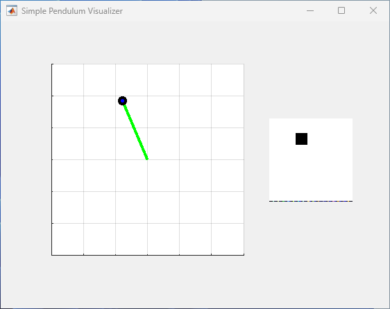
Environment Visualization

You can visualize the simple pendulum with image environment using the plot function. The main figure on the left side of the plot displays the rod as a green line, and a black circle surrounding a blue dot indicates the position of the rod center of mass. The plot also contains a smaller figure on the right visualizing the content of the first observation channel, which is a 50-by-50 pixel image with a black square representing the position of the pendulum center of mass.

plot(env)

To visualize the environment during training, call plot before training and keep the visualization figure open.

Note

While visualizing the environment during training might often be insightful, doing so tends to increase training time. For faster training, keep the environment plot closed during training.

Environment Properties

All the environment properties listed in this table are writable. You can change them to customize the simple pendulum with image environment to your needs.

Property	Description	Default
Mass	Pendulum mass in kilograms	1
RodLength	Distance from the hinge to the pendulum center of mass in meters. For uniform rods, this distance is the half-length.	1
RodInertia	Inertia moment of the rod (pendulum) about its center of mass in kilograms per meter squared	0
Gravity	Acceleration due to gravity in meters per second squared	9.81
DampingRatio	Damping on pendulum motion (viscous friction) in newtons per meter per second.	0
MaximumTorque	Maximum input torque in newtons per meter. If the magnitude of the input torque exceeds this threshold, the magnitude of the torque that is actually applied to the pendulum is limited to MaximumTorque	2
Ts	Sample time in seconds. The software uses the sample time to discretize the dynamics of the underlying continuous-time system. The discrete-time dynamics is then used to calculate the next state as a function of the current state and of the applied action.	0.05
State	Environment state, specified as a column vector with these state variables: Pendulum angle (counterclockwise-positive, radians) Pendulum angular velocity (radians per second)	[0 0 ]'
Q	Weight matrix for the observation component of reward signal	[1 0;0 0.1]
R	Weight matrix for the action component of reward signal	1e-3

Dynamics

The pendulum is a rigid rod subjected to an input torque (counterclockwise positive) and might be subjected to a viscous friction that counteracts the torque. The angle of rotation is counterclockwise positive and gravity acts vertically downwards. The center of gravity of the pendulum is at its half-length. The continuous-time equations used to model this system are described in the Simple Pendulum Equation section of the example Derive Equations of Motion and Simulate Cart-Pole System (Symbolic Math Toolbox). The discrete-time dynamics of the environment are then obtained using a trapezoidal integration method.

Actions

The agent interacts with the environment using an action channel carrying a single scalar, the torque applied at the base of the pendulum. The action space specification is as follows:

• For environments with a discrete action space, the specification is an rlFiniteSetSpec object.

  actInfo = getActionInfo(env)

    actInfo =
  
    rlFiniteSetSpec with properties:
  
         Elements: [-2 -1 0 1 2]
             Name: "torque"
      Description: [0×0 string]
        Dimension: [1 1]
         DataType: "double"

• For environments with a continuous action space, the specification is an rlNumericSpec object.

  actInfo = getActionInfo(env)

    actInfo =
  
    rlNumericSpec with properties:
  
       LowerLimit: -2
       UpperLimit: 2
             Name: "torque"
      Description: [0×0 string]
        Dimension: [1 1]
         DataType: "double"

For more information on obtaining action specifications from an environment, see getActionInfo.

Observations

In a simple pendulum environment with image environment, the agent receives the following observation signals:

• 50-by-50 grayscale image of the pendulum position

• Derivative of the pendulum angle

The observation has two channels, each specified by an rlNumericSpec object, because both signals are continuous.

obsInfo = getObservationInfo(env)

  1×2 rlNumericSpec array with properties:

    LowerLimit
    UpperLimit
    Name
    Description
    Dimension
    DataType

obsInfo(1)

  rlNumericSpec with properties:

     LowerLimit: 0
     UpperLimit: 1
           Name: "pendImage"
    Description: [0×0 string]
      Dimension: [50 50]
       DataType: "double"

obsInfo(2)

  rlNumericSpec with properties:

     LowerLimit: -Inf
     UpperLimit: Inf
           Name: "angularRate"
    Description: [0×0 string]
      Dimension: [1 1]
       DataType: "double"

For more information on obtaining observation specifications from an environment, see getObservationInfo.

Reward

The reward signal for this environment, at time t, is:

$$r_t=-\left({\theta }_t^2+0.1{\dot{\theta }}_t^2+0.001u_{t-1}^2\right)$$

Here:

• θ_t is the pendulum angle of displacement from the upright position (counterclockwise-positive, radians).

• $${\dot{\theta }}_t$$ is the derivative of the pendulum angle with respect to time.

• u_t–1 is the control effort from the previous time step.

Reset Function

The reset function sets the initial state of the environment so that the pendulum is hanging downward and still.

reset(env);
env.State

ans =

    3.1416
         0

Unlike other environments, you cannot set your own reset function for a simple pendulum with image environment.

Create a Default Agent for this Environment

The environment observation and action specifications allow you to create an agent that works with your environment. For example, for the discrete action space version of this environment, create a default DQN agent.

dqnAgent = rlDQNAgent(obsInfo,actInfo)

dqnAgent = 

  rlDQNAgent with properties:

        ExperienceBuffer: [1×1 rl.replay.rlReplayMemory]
            AgentOptions: [1×1 rl.option.rlDQNAgentOptions]
    UseExplorationPolicy: 0
         ObservationInfo: [1×2 rl.util.rlNumericSpec]
              ActionInfo: [1×1 rl.util.rlFiniteSetSpec]
              SampleTime: 1

If needed, modify the agent options using dot notation.

dqnAgent.AgentOptions.CriticOptimizerOptions.LearnRate = 1e-3;

You can now use both the environment and the agent as arguments for the built-in functions train and sim, which train or simulate the agent within the environment, respectively.

You can also create and train agents for this environment interactively using the Reinforcement Learning Designer app. For an example, see Design and Train Agent Using Reinforcement Learning Designer.

For more information on creating agents, see Reinforcement Learning Agents.

Step Function

You can also call the environment step function to return the next observation, reward, and an is-done scalar indicating whether a final state has been reached.

For example, call the step function with an input torque of 1 newton per meter.

[xn,rn,id]=step(env,1)

xn =

  1×2 cell array

    {50×50 double}    {[0.0500]}


rn =

   -9.8630


id =

  logical

   0

The environment step and reset functions allow you to create a custom training or simulation loop. For more information on custom training loops, see Train Reinforcement Learning Policy Using Custom Training Loop.

Environment Code

To access the functions that returns the discrete action space version of this environment, at the MATLAB command line, type:

edit rl.env.SimplePendlumWithImageDiscreteAction

To access the function that returns the continuous action space version of this environment, at the MATLAB command line, type:

edit rl.env.SimplePendlumWithImageContinuousAction

To access the abstract class that contains the step function, at the MATLAB command line, type:

edit rl.env.AbstractSimplePendlumWithImage

Simulink Simple Pendulum Swing-up Environment

A simple pendulum swing-up environment is a predefined Simulink environment featuring a simple pendulum that initially hangs still in a downward position (that is, the initial angle of the pendulum is π and its initial angular speed is zero). The goal of the agent is to swing up the pendulum by applying an input torque and then keep the pendulum upright using minimal control effort.

The model for this environment is defined in the rlSimplePendulumModel Simulink model.

open_system("rlSimplePendulumModel")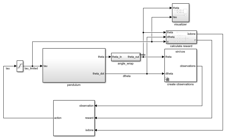

There are two simple pendulum environment variants, which differ by the agent action space.

• Discrete — The agent can apply a torque of either T_max, 0, or -T_max to the pendulum.

• Continuous — The agent can apply any torque within the range [-T_max,T_max].

Here, T_max is the variable max_tau, which you can change by accessing the workspace of the rlSimplePendulumModel model. For more information on other variables that you can change, see Dynamics. For more information on Simulink model workspaces, see Model Workspaces (Simulink) and Change Model Workspace Data (Simulink).

To create a simple pendulum environment, use the rlPredefinedEnv as follows, depending on the desired action space:

• Discrete action space:

  env = rlPredefinedEnv("SimplePendulumModel-Discrete")

  env = 
  
  SimulinkEnvWithAgent with properties:
  
             Model : rlSimplePendulumModel
        AgentBlock : rlSimplePendulumModel/RL Agent
          ResetFcn : []
    UseFastRestart : on

  For an example of how to that train an agent in this environment, see Train DQN Agent to Swing Up and Balance Pendulum. For an example comparing the most used discrete action space agents on this environment, see Compare Agents on the Discrete Pendulum Swing-Up Environment.

• Continuous action space:

  env = rlPredefinedEnv("SimplePendulumModel-Continuous")

  env = 
  
  SimulinkEnvWithAgent with properties:
  
             Model : rlSimplePendulumModel
        AgentBlock : rlSimplePendulumModel/RL Agent
          ResetFcn : []
    UseFastRestart : on
  

  For an example of how to that train an agent in this environment, see Train DDPG Agent to Swing Up and Balance Pendulum. For an example comparing the most used continuous action space agents on this environment, see Comparison of Agents on the Continuous Pendulum Swing-Up Environment.

Note

When training or simulating an agent within a Simulink environment, to ensure that the RL Agent block executes at the desired sample time, set the SampleTime property of the agent object appropriately.

For more information on Simulink environments, see SimulinkEnvWithAgent and Create Custom Simulink Environments.

Environment Visualization

The environment is visualized with a plot that displays the pendulum as a green line and a black circle surrounding a blue dot indicating the position of the rod center of mass. The plot is displayed automatically by the Simulink model when it is executed by the simulation or training function.

Environment Properties

The environment properties that you can access using dot notation are described in SimulinkEnvWithAgent.

Dynamics

The pendulum is a rigid rod subjected to an input counterclockwise-positive torque. The pendulum might be subjected to a viscous friction that counteracts the torque. The angle of rotation is counterclockwise positive and gravity acts vertically downward. The center of gravity of the pendulum is at its half-length. For the exact continuous-time equations used to model this system, see the Simple Pendulum Equation section in the example Derive Equations of Motion and Simulate Cart-Pole System (Symbolic Math Toolbox). During simulation, the Simulink solver then integrates the dynamics according to the selected solver, while the RL Agent block executes at discrete intervals according to the sample time specified in the SampleTime property of the agent.

The pendulum dynamics are represented in the pendulum subsystem of the rlSimplePendulumModel model, which calculates the pendulum angular position and velocity as a function of the input force and of the previous state:

The parameters that define the pendulum dynamics are stored in the workspace of the rlSimplePendulumModel model.

Variable	Description	Default
I	Inertia moment of the rod (pendulum) about its center of mass in kilograms per meter squared	0
c	Torque damping on pendulum motion (viscous friction) in newtons per meter per second.	0
g	Acceleration due to gravity in meters per second squared	9.81
l	Distance from the hinge to the pendulum center of mass in meters. For uniform rods, this distance is the half-length.	1
m	Pendulum mass in kilograms	1
max_tau	Maximum input torque in newtons per meter. If the magnitude of the input torque exceeds this threshold, the magnitude of the torque that is actually applied to the pendulum is limited to MaximumTorque.	2
theta0	Initial value of the pendulum angle (counterclockwise-positive). The reset function normally sets this value topi.	0
theta_dot0	Initial value of the pendulum angular speed. The reset function normally sets this value to 0.	0

For more information on Simulink model workspaces, see Model Workspaces (Simulink) and Change Model Workspace Data (Simulink).

Actions

The agent interacts with the environment using an action channel carrying a single scalar, the torque applied at the base of the pendulum. The action space specification is as follows:

• For an environment with a discrete action space, the specification is an rlFiniteSetSpec object.

  actInfo = getActionInfo(env)

  actInfo = 
  
    rlFiniteSetSpec with properties:
  
         Elements: [3×1 double]
             Name: "torque"
      Description: [0×0 string]
        Dimension: [1 1]
         DataType: "double"

  actInfo.Elements'

  ans =
  
      -2     0     2

• For an environment with a continuous action space, the specification is an rlNumericSpec object.

• actInfo = getActionInfo(env)

  actInfo = 
  
    rlNumericSpec with properties:
  
       LowerLimit: -2
       UpperLimit: 2
             Name: "torque"
      Description: [0×0 string]
        Dimension: [1 1]
         DataType: "double"

For more information on obtaining action specifications from an environment, see getActionInfo.

Observations

In a simple pendulum swing-up with Simulink environment, the observation is calculated within the create observations subsystem of the rlSimplePendulumModel model.

The agent receives these observation signals:

• Sine of the pendulum angle

• Cosine of the pendulum angle

• Derivative of the pendulum angle with respect to time

The observation has a single channel specified by an rlNumericSpec object, because the three observation signals are continuous.

obsInfo = getObservationInfo(env)

obsInfo = 

  rlNumericSpec with properties:

     LowerLimit: -Inf
     UpperLimit: Inf
           Name: "observations"
    Description: [0×0 string]
      Dimension: [3 1]
       DataType: "double"

For more information on obtaining observation specifications from an environment, see getObservationInfo.

Reward

In this environment, the reward is calculated within the calculate reward subsystem of the rlSimplePendulumModel model.

The reward is

$$r_t=-\left({\theta }_t^2+0.1{\dot{\theta }}_t^2+0.001u_{t-1}^2\right)$$

Here:

• θ_t is the pendulum angle of displacement (counterclockwise-positive) from the upright position.

• $${\dot{\theta }}_t$$ is the derivative of the pendulum angle with respect to time.

• u_t–1 is the control effort from the previous time step.

Reset Function

The environment has no default reset function. However, you can set your own reset function to set the initial state of the pendulum every time a simulation starts to train or simulate the environment.

For example, to set the initial condition of the pendulum as still and hanging downward, specify the handle of an anonymous reset function that sets the model workspace variable theta0 to pi.

env.ResetFcn = @(in)setVariable(in,
          "theta0",pi, ...
          "Workspace","rlSimplePendulumModel");

Here, you use setVariable (Simulink) to set the variable theta0 to a random value in the Simulink.SimulationInput (Simulink) object in. The value of theta0 that you specify overrides the existing theta0 value in the model workspace for the duration of the simulation or training. The value of theta0 then reverts to its original value when the simulation or training completes.

Create a Default Agent for this Environment

The environment observation and action specifications allow you to create an agent that works with your environment. For example, for the continuous action space version of this environment, create a default PPO agent.

agent = rlPPOAgent(obsInfo,actInfo)

agent = 

  rlPPOAgent with properties:

            AgentOptions: [1×1 rl.option.rlPPOAgentOptions]
    UseExplorationPolicy: 1
         ObservationInfo: [1×1 rl.util.rlNumericSpec]
              ActionInfo: [1×1 rl.util.rlNumericSpec]
              SampleTime: 1

Set the agent sample time so that the RL Agent block executes at the desired rate.

agent.SampleTime = 0.05;

If needed, modify the agent options using dot notation.

agent.AgentOptions.CriticOptimizerOptions.LearnRate = 1e-3;
agent.AgentOptions.ActorOptimizerOptions.LearnRate = 1e-3;

You can now use both the environment and the agent as arguments for the built-in functions train and sim, which train or simulate the agent within the environment, respectively.

You can also create and train agents for this environment interactively using the Reinforcement Learning Designer app. For an example, see Design and Train Agent Using Reinforcement Learning Designer.

For more information on creating agents, see Reinforcement Learning Agents.

Step Function

Because this is a Simulink environment, calling the step function is not supported. For an example on how to build a custom training loop using a Simulink environment, see Custom Training Loop with Simulink Action Noise.

Simscape Cart-Pole Swing-up Environment

A Simscape cart-pole swing-up environment is a predefined Simulink environment featuring a cart-pole system modeled using Simscape Multibody™. The pole initially hangs still in a downward position (that is, the initial angle is π radians and the initial angular speed is zero). The goal of the agent is to swing up the pole by applying an input force on the cart and then maintain the pole upright using minimal control effort. The episode terminates if the cart moves more than 3.5 meters from the original position.

The model for this environment is defined in the rlCartPoleSimscapeModel Simulink model.

open_system("rlCartPoleSimscapeModel")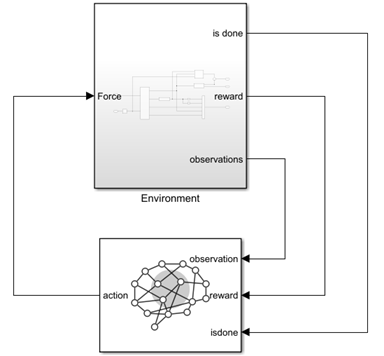

In the Environment subsystem, the model dynamics are defined within the Plant subsystem, using Simscape components. The reward and is-done signals are defined in the qr reward and x limit penalty subsystems, respectively, using Simulink blocks. The black multiplexer block aggregates the observations into a single observation signal.

open_system("rlCartPoleSimscapeModel/Environment")

There are two variants of this environment, which differ by the agent action space:

• Discrete — The agent can apply a force of 15, 0, or -15 newtons to the cart.

• Continuous — The agent can apply any force within the range [-15,15] newtons.

To create a cart-pole environment, use rlPredefinedEnv as follows, depending on the desired action space:

• Discrete action space:

  env = rlPredefinedEnv("CartPoleSimscapeModel-Discrete")

  env = 
  
  SimulinkEnvWithAgent with properties:
  
             Model : rlCartPoleSimscapeModel
        AgentBlock : rlCartPoleSimscapeModel/RL Agent
          ResetFcn : []
    UseFastRestart : on

  For an example comparing the most used discrete action space agents on this environment, see Compare Agents on the Discrete Simscape Cart-Pole Swing-Up Environment.

• Continuous action space:

  env = rlPredefinedEnv("CartPoleSimscapeModel-Continuous")

  env = 
  
  SimulinkEnvWithAgent with properties:
  
             Model : rlCartPoleSimscapeModel
        AgentBlock : rlCartPoleSimscapeModel/RL Agent
          ResetFcn : []
    UseFastRestart : on
  

  For an example that trains an agent in this cart-pole environment, see Train DDPG Agent to Swing Up and Balance Cart-Pole System. For an example comparing the most used discrete action space agents on this environment, see Compare Agents on the Continuous Cart Pole Swing-Up Environment.

Note

When training or simulating an agent within a Simulink environment, to ensure that the RL Agent block executes at the desired sample time, set the SampleTime property of the agent object appropriately.

For more information on Simulink environments, see SimulinkEnvWithAgent and Create Custom Simulink Environments.

Environment Visualization

The environment visualization shows the cart and the pole as gray and red rectangles, respectively, and it is displayed automatically in the Mechanics Explorer by the Simulink model when it is executed by the simulation or training function.

Environment Properties

The environment properties that you can access using dot notation are described in SimulinkEnvWithAgent.

Dynamics

The cart is subjected to an external input force as well as viscous friction and can move horizontally (the horizontal axis points right). The pole is not subject to friction and can rotate about the hinge on the cart (counterclockwise rotations are positive). Gravity acts vertically downwards. For the exact continuous-time equations used to model this system, see the Examples of Cart-Pole System in Simscape Multibody section in the example Derive Equations of Motion and Simulate Cart-Pole System (Symbolic Math Toolbox). During simulation, the Simulink solver integrates the dynamics according to the selected solver, while the RL Agent block executes at discrete intervals according to the sample time specified in the SampleTime property of the agent.

The continuous-time system dynamics are represented using Simscape Multibody in the Plant subsystem of the rlCartPoleSimscapeModel model. This subsystem calculates the linear and angular positions and velocities of the cart and pole, respectively, as a function of the input force on the cart and of the previous state:

The parameters that define the system dynamics are stored in the workspace of the rlCartPoleSimscapeModel model.

Variable	Description	Default
mCart	Mass of the cart in kilograms	1
mPend	Mass of the pole in kilograms	1
Gravity	Acceleration due to gravity in meters per second squared	9.8
Length	Distance from the pole hinge to the cart center of mass. If the pole density is uniform, this distance is half the length of the pole.	0.5
theta0	Initial value of the pendulum angle (counterclockwise-positive) in degrees.	180
Kd	Force damping on cart motion (viscous friction) in newtons per second over meter.	10

For more information on Simulink model workspaces, see Model Workspaces (Simulink) and Change Model Workspace Data (Simulink).

Actions

The agent interacts with the environment using an action channel carrying a single scalar, the horizontal force applied to the cart. The action space specification is as follows:

• Discrete action space, the channel is specified by an rlFiniteSetSpec object.

  actInfo = getActionInfo(env)

  actInfo = 
  
    rlFiniteSetSpec with properties:
  
         Elements: [3×1 double]
             Name: "force"
      Description: [0×0 string]
        Dimension: [1 1]
         DataType: "double"

  actInfo.Elements'

  ans =
  
     -15     0    15

• Continuous action space, the channel is specified by an rlNumericSpec object.

  actInfo = getActionInfo(env)

  actInfo = 
  
    rlNumericSpec with properties:
  
       LowerLimit: -15
       UpperLimit: 15
             Name: "force"
      Description: [0×0 string]
        Dimension: [1 1]
         DataType: "double"

For more information on obtaining action specifications from an environment, see getActionInfo.

Observations

In this environment, the observations are aggregated using a multiplexer block within the Environment subsystem of the rlCartPoleSimscapeModel model. The agent receives the following five observation signals.

• Sine of the pole angle

• Cosine of the pole angle

• Derivative of the pendulum angle

• Cart position

• Derivative the of cart position

The observation has a single channel, specified by an rlNumericSpec object, because the five observation signals are continuous,

obsInfo = getObservationInfo(env)

obsInfo = 

  rlNumericSpec with properties:

     LowerLimit: -Inf
     UpperLimit: Inf
           Name: "observations"
    Description: [0×0 string]
      Dimension: [5 1]
       DataType: "double"

For more information on obtaining observation specifications from an environment, see getObservationInfo.

Reward

In this environment, the reward is calculated within the qr reward subsystem.

The reward signal for this environment is the sum of two components (r = r_qr + r_n + r_p):

• A quadratic regulator control reward, constructed in the Environment/qr reward subsystem:

  $$r_{qr}=-\left(0.1\ast x^2+0.5\ast {\theta }^2+0.005\ast u_{t-1}^2\right)$$

• A cart limit penalty, constructed in the Environment/x limit penalty subsystem. This subsystem generates a negative reward when the magnitude of the cart position exceeds a given threshold:

  $$r_p=-100\ast \left(\left|x\right|\ge 3.5\right)$$

Here:

• x is the cart position.

• θ is the pole angle of displacement from the upright position.

• u_t–1 is the control effort from the previous time step.

Reset Function

The environment has no default reset function. However, you can set your own reset function to set the initial state of the system every time a simulation starts to train or simulate the environment.

For example, to set the initial pole to a random angle between 180 and –180 degrees, instead of the default value of 180 degrees, specify the handle of an anonymous reset function that sets the model workspace variable theta0 to 360*rand-180.

env.ResetFcn = @(in)setVariable(in, ...
          "theta0",360*rand-180, ...
          "Workspace","rlCartPoleSimscapeModel");

Here, you use setVariable (Simulink) to set the variable theta0 to a random value in the Simulink.SimulationInput (Simulink) object in. The value of theta0 that you specify overrides the existing theta0 value in the model workspace for the duration of the simulation or training. The value of theta0 then reverts to its original value when the simulation or training completes.

Create a Default Agent for this Environment

The environment observation and action specifications allow you to create an agent that works with your environment. For example, for the discrete action space version of this environment, create a default SAC agent.

agent = rlSACAgent(obsInfo,actInfo)

agent = 

  rlSACAgent with properties:

        ExperienceBuffer: [1×1 rl.replay.rlReplayMemory]
            AgentOptions: [1×1 rl.option.rlSACAgentOptions]
    UseExplorationPolicy: 1
         ObservationInfo: [1×1 rl.util.rlNumericSpec]
              ActionInfo: [1×1 rl.util.rlFiniteSetSpec]
              SampleTime: 1

Set the agent sample time so that the RL Agent block executes at the desired rate.

agent.SampleTime = 0.02;

If needed, modify the agent options using dot notation.

agent.AgentOptions.CriticOptimizerOptions(1).LearnRate = 1e-3;
agent.AgentOptions.CriticOptimizerOptions(2).LearnRate = 1e-3;
agent.AgentOptions.ActorOptimizerOptions.LearnRate = 1e-3;

You can now use both the environment and the agent as arguments for the built-in functions train and sim, which train or simulate the agent within the environment, respectively.

You can also create and train agents for this environment interactively using the Reinforcement Learning Designer app. For an example, see Design and Train Agent Using Reinforcement Learning Designer.

For more information on creating agents, see Reinforcement Learning Agents.

Step Function

Because this is a Simulink environment, calling the step function is not supported. For an example on how to build a custom training loop using a Simulink environment, see Custom Training Loop with Simulink Action Noise.