振動信号を使用した状態の監視と予知

ライブスクリプトを開く

この例では、ボールベアリングの振動信号から特徴を抽出し、健全性を監視して、予知を行う方法を示します。この例では、Signal Processing Toolbox™ および System Identification Toolbox™ の機能を使用し、Predictive Maintenance Toolbox™ は必要ありません。

データの説明

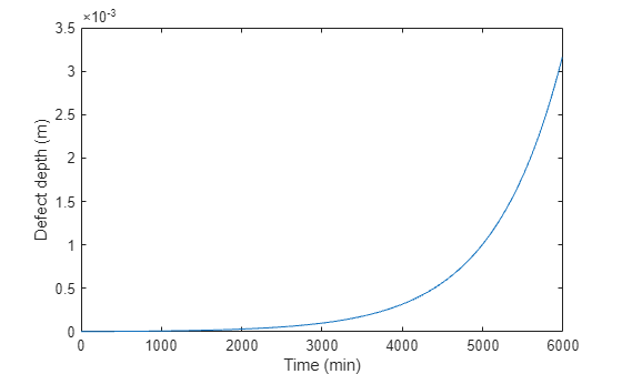
pdmBearingConditionMonitoringData.mat に保存された振動データを読み込みます (これは最大 88 MB の大規模なデータセットで、MathWorks サポートファイルサイトで入手します)。データは cell 配列に格納されています。これは、ベアリングの外輪上に単一点の欠陥をもつボールベアリング信号シミュレーターを使用して生成されたものです。異なる健康状態 (欠陥が 3um から 3mm を超える深さまで増加) でシミュレートしたベアリングの振動信号のセグメントが複数含まれています。各セグメントにはサンプリングレート 20 kHz で 1 秒間に収集された信号が含まれます。pdmBearingConditionMonitoringData.mat では、欠陥の深さが時間とともにどのように変化するかが defectDepthVec に保存され、その対応する時間が expTime に分単位で保存されています。

url = 'https://www.mathworks.com/supportfiles/predmaint/condition-monitoring-and-prognostics-using-vibration-signals/pdmBearingConditionMonitoringData.mat';
websave('pdmBearingConditionMonitoringData.mat',url);
load pdmBearingConditionMonitoringData.mat

% Define the number of data points to be processed.
numSamples = length(data);

% Define sampling frequency.
fs = 20E3;          % unit: Hz

異なるデータセグメントで欠陥の深さがどのように変化するかをプロットします。

plot(expTime,defectDepthVec);
xlabel('Time (min)');
ylabel('Defect depth (m)');

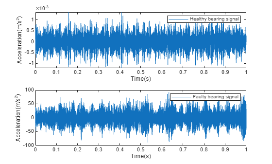
健全な状態のデータと故障状態のデータをプロットします。

time = linspace(0,1,fs)';

% healthy bearing signal
subplot(2,1,1);
plot(time,data{1});
xlabel('Time(s)');
ylabel('Acceleration(m/s^2)');
legend('Healthy bearing signal');

% faulty bearing signal
subplot(2,1,2);
plot(time,data{end});
xlabel('Time(s)');
ylabel('Acceleration(m/s^2)');
legend('Faulty bearing signal');

特徴抽出

この節では、データの各セグメントから代表的な特徴を抽出します。これらの特徴は健全性の監視と予知に使用されます。ベアリングの診断と予知のための代表的な特徴には、時間領域の特徴 (平方根平均二乗、ピーク値、信号尖度など) または周波数領域の特徴 (ピーク周波数、周波数平均など) が含まれます。

使用する特徴を選択する前に、振動信号のスペクトログラムをプロットします。時間領域または周波数領域、あるいは時間-周波数領域での信号を可視化すると、劣化や故障を示す信号パターンを見つけるのに役立ちます。

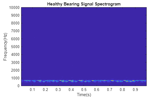
まず、健全なベアリングデータのスペクトログラムを計算します。ウィンドウサイズ 500 データ点、オーバーラップ率 90% (450 データ点と等価) を使用します。FFT の点の数を 512 に設定します。fs は前に定義したサンプリング周波数を表します。

[~,fvec,tvec,P0] = spectrogram(data{1},500,450,512,fs);

P0 はスペクトログラム、fvec は周波数ベクトル、tvec は時間ベクトルです。

健全なベアリング信号のスペクトログラムをプロットします。

clf;
imagesc(tvec,fvec,P0)
xlabel('Time(s)');
ylabel('Frequency(Hz)');
title('Healthy Bearing Signal Spectrogram');
axis xy

次に、故障のパターンが生じた振動信号のスペクトログラムをプロットします。高周波数で信号エネルギーが集中しているのがわかります。

[~,fvec,tvec,Pfinal] = spectrogram(data{end},500,450,512,fs);
imagesc(tvec,fvec,Pfinal)
xlabel('Time(s)');
ylabel('Frequency(Hz)');
title('Faulty Bearing Signal Spectrogram');
axis xy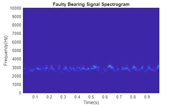

健全な状態のベアリングと故障状態のベアリングから得たデータのスペクトログラムは異なっているので、スペクトログラムから代表的な特徴を抽出し、状態の監視と予知に利用できます。この例では、健康インジケーターとしてスペクトログラムからピーク周波数平均を抽出します。スペクトログラムを $P (t, ω)$ と表します。各時間インスタンスでのピーク周波数は次のように定義されます。

$P e a k F r e q (t) = a r g m a x_{ω} P (t, ω)$

ピーク周波数平均は、上記で定義されたピーク周波数の平均です。

$m e a n P e a k F r e q = \frac{1}{T} \int_{0}^{T} P e a k F r e q (t) d t$

健全なボールベアリング信号のピーク周波数平均を計算します。

[~,I0] = max(P0);               % Find out where the peak frequencies are located.
meanPeakFreq0 = mean(fvec(I0))  % Calculate mean peak frequency.

meanPeakFreq0 = 666.4602

健全なベアリング振動信号の場合、ピーク周波数平均は約 650 Hz です。次に、故障のあるベアリング信号のピーク周波数平均を計算します。ピーク周波数平均が 2500 Hz を超える値にシフトします。

[~,Ifinal] = max(Pfinal);
meanPeakFreqFinal = mean(fvec(Ifinal))

meanPeakFreqFinal = 2.8068e+03

欠陥がそれほど深くなく、ただし、振動信号への影響が出始めている中間段階におけるデータを調べます。

[~,fvec,tvec,Pmiddle] = spectrogram(data{end/2},500,450,512,fs);
imagesc(tvec,fvec,Pmiddle)
xlabel('Time(s)');
ylabel('Frequency(Hz)');
title('Bearing Signal Spectrogram');
axis xy

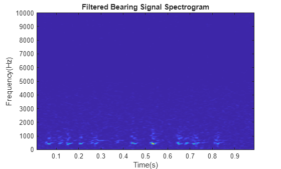
高周波数のノイズ成分はスペクトログラム全体に拡散しています。この現象は、元の振動とわずかな欠陥により生じた振動の両方の混合効果です。ピーク周波数平均を正確に計算するためには、データをフィルター処理してこれらの高周波数成分を取り除きます。

振動信号にメディアンフィルターを適用して、高周波数の有用な情報は維持したまま高周波数のノイズ成分を除去します。

dataMiddleFilt = medfilt1(data{end/2},3);

メディアンフィルター処理の後でスペクトログラムをプロットします。高周波数成分が抑制されます。

[~,fvec,tvec,Pmiddle] = spectrogram(dataMiddleFilt,500,450,512,fs);
imagesc(tvec,fvec,Pmiddle)
xlabel('Time(s)');
ylabel('Frequency(Hz)');
title('Filtered Bearing Signal Spectrogram');
axis xy

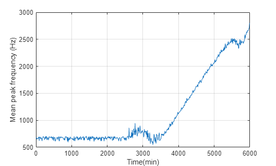
ピーク周波数平均によって健全なボールベアリングと故障したボールベアリングを正しく区別できるので、データの各セグメントからピーク周波数平均を抽出します。

% Define a progress bar.
h = waitbar(0,'Start to extract features');
% Initialize a vector to store the extracted mean peak frequencies.
meanPeakFreq = zeros(numSamples,1);
for k = 1:numSamples
    % Get most up-to-date data.
    curData = data{k};
    % Apply median filter.
    curDataFilt = medfilt1(curData,3);
    % Calculate spectrogram.
    [~,fvec,tvec,P_k] = spectrogram(curDataFilt,500,450,512,fs);
    % Calculate peak frequency at each time instance.
    [~,I] = max(P_k);
    meanPeakFreq(k) = mean(fvec(I));
    % Show progress bar indicating how many samples have been processed.
    waitbar(k/numSamples,h,'Extracting features');
end
close(h);

抽出したピーク周波数平均を時間に対してプロットします。

plot(expTime,meanPeakFreq);
xlabel('Time(min)');
ylabel('Mean peak frequency (Hz)');
grid on;

状態の監視と予知

この節では、事前定義されたしきい値と動的モデルを使用して状態の監視と予知を行います。状態監視のために、ピーク周波数平均が事前定義されたしきい値を超えた場合にトリガーされるアラームを作成します。予知を行うには、以降数時間のピーク周波数平均値を予想するための動的モデルを同定します。予想のピーク周波数平均が事前定義されたしきい値を超えた場合にトリガーされるアラームを作成します。

予想は、潜在的な故障に対する準備をしたり、故障が起きる前にマシンを停止したりする役に立ちます。ピーク周波数平均を時系列として考えてみましょう。ピーク周波数平均について時系列モデルを推定し、そのモデルを使って将来値を予想することができます。ピーク周波数平均の最初の 200 値を使用して初期の時系列モデルを作成してから、10 個の新しい値が利用可能になった時点で最後の 100 値を使用して時系列モデルを更新します。このようにバッチモードで時系列モデルを更新することにより、瞬間のトレンドを捉えることができます。更新された時系列モデルを使用して、10 ステップ先の予想を計算できます。

tStart = 200;               % Start Time
timeSeg = 100;              % Length of data for building dynamic model
forecastLen = 10;           % Define forecast time horizon
batchSize = 10;             % Define batch size for updating the dynamic model

予知と状態監視を行うには、マシンを停止するタイミングを決定するしきい値を設定する必要があります。この例では、シミュレーションで生成された健全なベアリングと故障のあるベアリングの統計データを使用して、しきい値を判定します。pdmBearingConditionMonitoringStatistics.mat には、健全なベアリングと故障のあるベアリングのピーク周波数平均の確率分布が保存されています。確率分布を計算するには、健全なベアリングと故障のあるベアリングの欠陥の深さに摂動を与えます。

url = 'https://www.mathworks.com/supportfiles/predmaint/condition-monitoring-and-prognostics-using-vibration-signals/pdmBearingConditionMonitoringStatistics.mat';
websave('pdmBearingConditionMonitoringStatistics.mat',url);
load pdmBearingConditionMonitoringStatistics.mat

健全なベアリングと故障のあるベアリングのピーク周波数平均の確率分布をプロットします。

plot(pFreq,pNormal,'g--',pFreq,pFaulty,'r');
xlabel('Mean peak frequency(Hz)');
ylabel('Probability Distribution');
legend('Normal Bearing','Faulty Bearing');

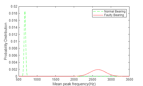
このプロットに基づいて、ピーク周波数平均のしきい値を 2000 Hz に設定して正常なベアリングと故障のあるベアリングを区別し、ベアリングの使用を最大化します。

threshold = 2000;

サンプリング時間を計算し、その単位を秒に変換します。

samplingTime = 60*(expTime(2)-expTime(1));                  % unit: seconds
tsFeature = iddata(meanPeakFreq(1:tStart),[],samplingTime);

ピーク周波数平均データの最初の 200 個をプロットします。

plot(tsFeature.y)

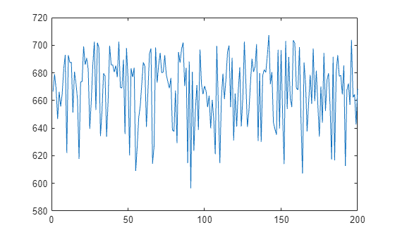
プロットを見ると、初期データが一定レベルとノイズの組み合わせであることがわかります。初期のベアリングは健全な状態にあり、ピーク周波数平均に大きな変化は予測されないため、これは期待どおりの動作です。

最初の 200 のデータ点を使用して 2 次状態空間モデルを同定します。モデルを正準形で取得し、サンプリング時間を指定します。

past_sys = ssest(tsFeature,2,'Ts',samplingTime,'Form','canonical')

past_sys =
  Discrete-time identified state-space model:
    x(t+Ts) = A x(t) + K e(t)
       y(t) = C x(t) + e(t)
 
  A = 
            x1       x2
   x1        0        1
   x2   0.9605  0.03942
 
  C = 
       x1  x2
   y1   1   0
 
  K = 
              y1
   x1  -0.003899
   x2   0.003656
 
Sample time: 600 seconds
  
Parameterization:
   CANONICAL form with indices: 2.
   Disturbance component: estimate
   Number of free coefficients: 4
   Use "idssdata", "getpvec", "getcov" for parameters and their uncertainties.

Status:                                               
Estimated using SSEST on time domain data "tsFeature".
Fit to estimation data: 0.2763% (prediction focus)    
FPE: 640, MSE: 602.7

初期に推定された動的モデルでは高い適合度が得られません。適合度のメトリクスは正規化平方根平均二乗誤差 (NRMSE) で、次のように計算されます。

$N R M S E = 1 - \frac{‖ x_{t r u e} - x_{p r e d} ‖}{‖ x_{t r u e} - m e a n (x_{t r u e}) ‖}$

ここで $x_{t r u e}$ は真の値、 $x_{p r e d}$ は予測された値です。

推定データが一定レベルとノイズとの組み合わせの場合、 $x_{p r e d} \approx m e a n (x_{t r u e})$ であり、NRMSE は 0 に近くなります。モデルを検証するには、残差の自己相関をプロットします。

resid(tsFeature,past_sys)

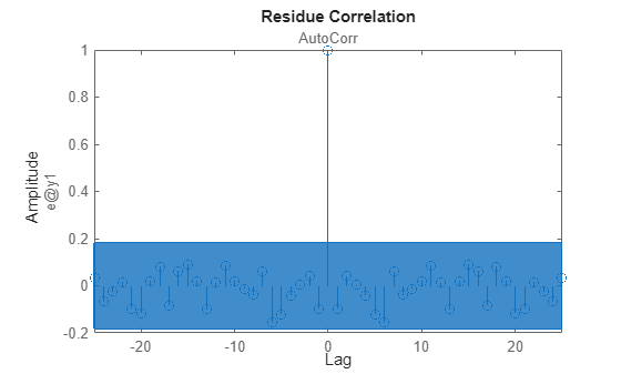
ここに示すように、残差は無相関であり、生成されたモデルは有効です。

同定されたモデル past_sys を使用してピーク周波数平均値を予想し、予想値の標準偏差を計算します。

[yF,~,~,yFSD] = forecast(past_sys,tsFeature,forecastLen);

予想値と信頼区間をプロットします。

tHistory = expTime(1:tStart);
forecastTimeIdx = (tStart+1):(tStart+forecastLen);
tForecast = expTime(forecastTimeIdx);

% Plot historical data, forecast value and 95% confidence interval.
plot(tHistory,meanPeakFreq(1:tStart),'b',...
     tForecast,yF.OutputData,'kx',...
     [tHistory; tForecast], threshold*ones(1,length(tHistory)+forecastLen), 'r--',...
     tForecast,yF.OutputData+1.96*yFSD,'g--',...
     tForecast,yF.OutputData-1.96*yFSD,'g--');

ylim([400, 1.1*threshold]);
ylabel('Mean peak frequency (Hz)');
xlabel('Time (min)');
legend({'Past Data', 'Forecast', 'Failure Threshold', '95% C.I'},...
    'Location','northoutside','Orientation','horizontal');
grid on;

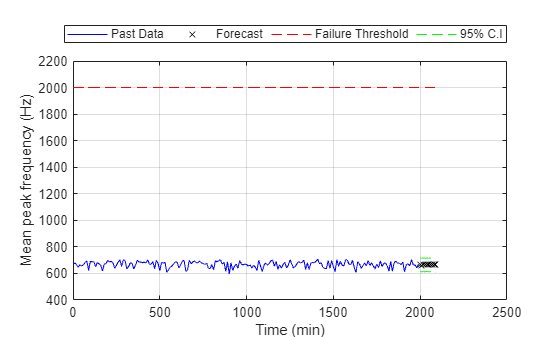
プロットを見ると、ピーク周波数平均の予想値がしきい値をはるかに下回っていることがわかります。

次に、新しいデータが利用可能になった時点でモデルパラメーターを更新し、予想値を再び推定します。また、信号や予想値が故障のしきい値を超えていないかどうかをチェックするためのアラームを作成します。

for tCur = tStart:batchSize:numSamples
    %  latest features into iddata object.
    tsFeature = iddata(meanPeakFreq((tCur-timeSeg+1):tCur),[],samplingTime);
    
    % Update system parameters when new data comes in. Use previous model
    % parameters as initial guesses.
    sys = ssest(tsFeature,past_sys);
    past_sys = sys;
    
    % Forecast the output of the updated state-space model. Also compute
    % the standard deviation of the forecasted output.
    [yF,~,~,yFSD]  = forecast(sys, tsFeature, forecastLen);
    
    % Find the time corresponding to historical data and forecasted values.
    tHistory = expTime(1:tCur);
    forecastTimeIdx = (tCur+1):(tCur+forecastLen);
    tForecast = expTime(forecastTimeIdx);
    
    % Plot historical data, forecasted mean peak frequency value and 95%
    % confidence interval.
    plot(tHistory,meanPeakFreq(1:tCur),'b',...
              tForecast,yF.OutputData,'kx',...
              [tHistory; tForecast], threshold*ones(1,length(tHistory)+forecastLen), 'r--',...
              tForecast,yF.OutputData+1.96*yFSD,'g--',...
              tForecast,yF.OutputData-1.96*yFSD,'g--');

    ylim([400, 1.1*threshold]);
    ylabel('Mean peak frequency (Hz)');
    xlabel('Time (min)');
    legend({'Past Data', 'Forecast', 'Failure Threshold', '95% C.I'},...
           'Location','northoutside','Orientation','horizontal');
    grid on;
    
    % Display an alarm when actual monitored variables or forecasted values exceed
    % failure threshold.
    if(any(meanPeakFreq(tCur-batchSize+1:tCur)>threshold))
        disp('Monitored variable exceeds failure threshold');
        break;
    elseif(any(yF.y>threshold))
        % Estimate the time when the system will reach failure threshold.
        tAlarm = tForecast(find(yF.y>threshold,1));
        disp(['Estimated to hit failure threshold in ' num2str(tAlarm-tHistory(end)) ' minutes from now.']);
        break;
    end
end

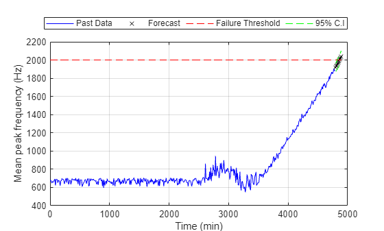
Estimated to hit failure threshold in 80 minutes from now.

最新の時系列モデルを確認します。

sys

sys =
  Discrete-time identified state-space model:
    x(t+Ts) = A x(t) + K e(t)
       y(t) = C x(t) + e(t)
 
  A = 
           x1      x2
   x1       0       1
   x2  0.2624   0.746
 
  C = 
       x1  x2
   y1   1   0
 
  K = 
           y1
   x1  0.3902
   x2  0.3002
 
Sample time: 600 seconds
  
Parameterization:
   CANONICAL form with indices: 2.
   Disturbance component: estimate
   Number of free coefficients: 4
   Use "idssdata", "getpvec", "getcov" for parameters and their uncertainties.

Status:                                               
Estimated using SSEST on time domain data "tsFeature".
Fit to estimation data: 92.53% (prediction focus)     
FPE: 499.3, MSE: 442.7

適合度が 90% を上回り、トレンドを正しく捉えることができています。

まとめ

この例では、測定されたデータから特徴を抽出して状態の監視と予知を実行する方法を示しました。抽出した特徴に基づいて動的モデルを生成および検証し、実際に故障が発生する前に対処できるよう、このモデルを使って故障が起きる時間を予想しました。

振動信号を使用した状態の監視と予知

データの説明

特徴抽出

状態の監視と予知

まとめ

関連するトピック