lsqcurvefit の勾配の確認

勾配評価関数を指定すると、lsqcurvefit などの非線形最小二乗ソルバーは、実行の速度および信頼性が向上する場合があります。ただし、勾配を確認するための lsqcurvefit ソルバーの構文は、他のソルバーと比べてわずかに異なります。

近似問題と checkGradient の構文

lsqcurvefit の勾配を確認するには、初期点 x0 を配列として渡すのではなく、cell 配列 {x0,xdata} を渡します。たとえば、応答関数 $$y=a+b\exp (-cx)$$ について、ノイズを追加したモデルからデータ ydata を作成します。応答関数は fitfun です。

function [F,J] = fitfun(x,xdata)
F = x(1) + x(2)*exp(-x(3)*xdata);
if nargout > 1
    J = [ones(size(xdata)) exp(-x(3)*xdata) -xdata.*x(2).*exp(-x(3)*xdata)];
end
end

xdata を 0 ～ 10 のランダムな点として作成し、ydata を応答と追加ノイズとして作成します。

a = 2;
b = 5;
c = 1/15;
N = 100;
rng default
xdata = 10*rand(N,1);
fun = @fitfun;
ydata = fun([a,b,c],xdata) + randn(N,1)/10;

応答関数の勾配が点 [a,b,c] で正しいことを確認します。

[valid,err] = checkGradients(@fitfun,{[a b c] xdata})

valid = logical
   1

err = struct with fields:
    Objective: [100×3 double]

指定した目的関数の勾配を問題なく使用できます。すべてのパラメーターの下限を 0 に設定し、上限は指定しません。

options = optimoptions("lsqcurvefit",SpecifyObjectiveGradient=true);
lb = zeros(1,3);
ub = [];
[sol,res,~,eflag,output] = lsqcurvefit(fun,[1 2 1],xdata,ydata,lb,ub,options)

Local minimum possible.

lsqcurvefit stopped because the final change in the sum of squares relative to 
its initial value is less than the value of the function tolerance.

<stopping criteria details>

sol = 1×3

    2.5872    4.4376    0.0802

res = 
1.0096

eflag = 
3

output = struct with fields:
      firstorderopt: 4.4156e-06
         iterations: 25
          funcCount: 26
       cgiterations: 0
          algorithm: 'trust-region-reflective'
           stepsize: 1.8029e-04
            message: 'Local minimum possible.↵↵lsqcurvefit stopped because the final change in the sum of squares relative to ↵its initial value is less than the value of the function tolerance.↵↵<stopping criteria details>↵↵Optimization stopped because the relative sum of squares (r) is changing↵by less than options.FunctionTolerance = 1.000000e-06.'
       bestfeasible: []
    constrviolation: []

lsqcurvefit の非線形制約関数

非線形制約関数で必要となる構文は、lsqcurvefit 目的関数の構文とは異なります。勾配のある非線形制約関数の形式は次のとおりです。

function [c,ceq,gc,gceq] = ccon(x)
c = ...
ceq = ...
if nargout > 2
    gc = ...
    gceq = ...
end
end

勾配の式のサイズは N 行 Nc 列にする必要があります。ここで、N は問題変数の数、Nc は制約関数の数です。たとえば、次の ccon 関数は非線形不等式制約を 1 つだけもちます。そのため、この関数は、3 つの変数をもつ次の問題についてサイズが 3 行 1 列の勾配を返します。

function [c,ceq,gc,gceq] = ccon(x)
ceq = [];
c = x(1)^2 + x(2)^2 + 1/x(3)^2 - 50;
if nargout > 2
    gceq = [];
    gc = zeros(3,1); % Gradient is a column vector
    gc(1) = 2*x(1);
    gc(2) = 2*x(2);
    gc(3) = -2/x(3)^3;
end
end

ccon 関数が点 [a,b,c] で正しい勾配を返すかどうかを確認します。

[valid,err] = checkGradients(@ccon,[a b c],IsConstraint=true)

valid = 1×2 logical array

   1   1

err = struct with fields:
    Inequality: [3×1 double]
      Equality: []

制約の勾配を使用するには、勾配関数を使用するオプションを設定し、非線形制約を使用して問題を再度解きます。

options.SpecifyConstraintGradient = true;
[sol2,res2,~,eflag2,output2] = lsqcurvefit(@fitfun,[1 2 1],xdata,ydata,lb,ub,[],[],[],[],@ccon,options)

Local minimum found that satisfies the constraints.

Optimization completed because the objective function is non-decreasing in 
feasible directions, to within the value of the optimality tolerance,
and constraints are satisfied to within the value of the constraint tolerance.

<stopping criteria details>

sol2 = 1×3

    4.4436    2.8548    0.2127

res2 = 
2.2623

eflag2 = 
1

output2 = struct with fields:
         iterations: 15
          funcCount: 22
    constrviolation: 0
           stepsize: 1.7914e-06
          algorithm: 'interior-point'
      firstorderopt: 3.3350e-06
       cgiterations: 0
            message: 'Local minimum found that satisfies the constraints.↵↵Optimization completed because the objective function is non-decreasing in ↵feasible directions, to within the value of the optimality tolerance,↵and constraints are satisfied to within the value of the constraint tolerance.↵↵<stopping criteria details>↵↵Optimization completed: The relative first-order optimality measure, 1.621619e-07,↵is less than options.OptimalityTolerance = 1.000000e-06, and the relative maximum constraint↵violation, 0.000000e+00, is less than options.ConstraintTolerance = 1.000000e-06.'
       bestfeasible: [1×1 struct]

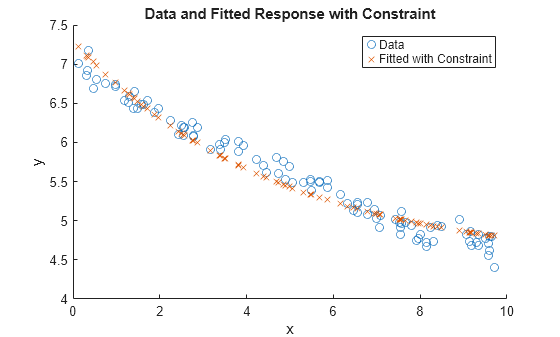
残差 res2 は、非線形制約がない残差 res の 2 倍を上回っています。この結果から、非線形制約によって解と制約なしの最小値に差が生じていることがわかります。

非線形制約を課す場合と課さない場合の解をプロットします。

scatter(xdata,ydata)
hold on
scatter(xdata,fitfun(sol,xdata),"x")
hold off
xlabel("x")
ylabel("y")
legend("Data","Fitted")
title("Data and Fitted Response, No Constraint")

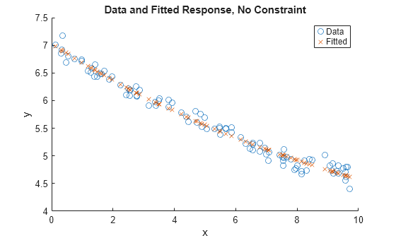
figure
scatter(xdata,ydata)
hold on
scatter(xdata,fitfun(sol2,xdata),"x")
hold off
xlabel("x")
ylabel("y")
legend("Data","Fitted with Constraint")
title("Data and Fitted Response with Constraint")

参考

checkGradients | lsqcurvefit

トピック

• lsqcurvefit を使用した非線形曲線近似
• 非線形最小二乗法とヤコビアンの有無