Control Mass-Spring-Damper System Using Data-Driven MPC

This example shows how to design and implement a data-driven model predictive controller to provide position tracking control for a mass-spring-damper system. Compared to classical MPC design, data-driven MPC design does not require a parametric plant model either from first principles or from system identification. Instead, it uses one set of input-output trajectory data directly as a non-parametric model for prediction, thereby enabling a much faster control system design process.

Mass-Spring-Damper Model

The plant for this example is a mass-spring-damper, consisting of two carts of mass $m_1$ and $m_2$, connected to each other and the ground through springs with the stiffness coefficients $c_0$ and $c_1$ and dampers with the damping coefficient $$d$$.

The linear time invariant model of the plant is as follows:

$\underset{}{\overset{\dot{}}{x\left(t\right)}}=Ax\left(t\right)+Bu\left(t\right)andy\left(t\right)=Cx\left(t\right)+Du\left(t\right)$ with

$$A=\left[\begin{array}{cccc}0& 1& 0& 0\\ -\frac{\left(c_0+c_1\right)}{m_1}& -\frac{2d}{m_1}& \frac{c_1}{m_1}& \frac{d}{m_1}\\ 0& 0& 0& 1\\ \frac{c_1}{m_2}& \frac{d}{m_2}& -\frac{c_1}{m_2}& -\frac{d}{m_2}\end{array}\right],B=\left[\begin{array}{c}0\\ 0\\ 0\\ \frac{1}{m_2}\end{array}\right],C=\left[0010\right],D=0$$

where:

• $x=\left[p_1,\underset{}{\overset{\dot{}}{p_1}},p_2,\underset{}{\overset{\dot{}}{p_2}}\right]$ is the system state vector.

• $p_1$ and $p_2$ are the positions of the masses and only $p_2$ is measured.

• The external force $F$ is the control action.

The goal of the controller is to manipulate $F$ so that $p_2$ tracks a reference.

Set the system parameters.

% stiffness
c0 = 1;
c1 = 1;
% damping
d = 1;
% mass
m1 = 5;
m2 = 1;

Create the state-space model of the system equations.

A = [0 1 0 0;
    -(c0+c1)/m1 -2*d/m1 c1/m1 d/m1;
    0 0 0 1;
    c1/m2 d/m2 -c1/m2 -2*d/m2];
B = [0; 0; 0; 1/m2];
C = [0 0 1 0];
D = 0;
sys = ss(A,B,C,D);

Extract the dimensions.

[ny,nu] = size(D);
nx = order(sys);

Set the initial state, output and input.

x0 = zeros(nx,1);
y0 = zeros(ny,1);
u0 = zeros(nu,1);

Collect Input and Output Data From Plant Model

Set up the the data collection experiment parameters.

rng(12345);         % random number seed
Ts = 0.1;           % sample time
N = 61;             % experiment length (6 seconds)
t = (0:N-1)'*Ts;    % time vector

Generate the data. Define the input trajectory as a series of random numbers, and use lsim to obtain the corresponding output trajectory.

dataU = (0.5-rand(length(t),1))*2;
dataY = lsim(sys,dataU,t,x0);

Add a small measurement noise to the output data.

dataY = dataY .*(1+(rand(size(dataY))-0.5)*0.01);

Data-Driven MPC Design

The main steps of data-driven MPC design are as follows:

1. Create the DataDrivenMPC object and specify appropriate future steps, past steps, and plant order parameters.

2. Verify the quality of the collected data by checking the persistentExcitation property.

3. Assess the accuracy of the prediction model by using checkPrediction.

4. Specify bounds and weights.

5. Simulate the closed loop response.

Create DataDrivenMPC Object and Specify Main Design Parameters

Create the DataDrivenMPC object ddobj using the input and output data as well as the sample time at which they were collected.

ddobj = DataDrivenMPC(dataU,dataY,Ts);

Specify the FutureSteps property. This value is usually determined by your control objective.

Since data-driven MPC includes the current time k as part of the prediction, the FutureSteps property is equivalent to the PredictionHorizon property of classical MPC (which predicts from time k + 1 to k + N) plus 1.

ddobj.FutureSteps = 21;

Specify the PastSteps property. This value indicates how far into the past history of the input-output trajectory that the data-driven MPC needs to rely on to obtain a good estimation of the current plant state, which is important for prediction.

In general, however, choosing PastSteps might require some trial and error:

• If the value is too small, a correct estimation of the current plant state is not possible.

• If the value is too large, the size of the optimization problem increases and overfitting can occur.

ddobj.PastSteps = 4;

Specify the PlantOrder property. This value is usually determined by your knowledge of the specific plant.

Like with PastSteps, choosing a PlantOrder value might require some trial and error. Typically the value is the number of the plant poles (modes) that are significant to your control problem.

ddobj.PlantOrder = 4;

After FutureSteps, PastSteps and PlantOrder are selected, take the following two actions to assess the quality of the data set and validate whether the data set can work with your choices.

Assess Data Quality

To assess the quality of the collected data, check the PersistentExcitation Property

ddobj.PersistentExcitation

ans = struct with fields:
           NumberOfSamples: 61
    MinimumNumberOfSamples: 57
               HankelDepth: 25
        MaximumHankelDepth: 27
          IsDataSufficient: 1
    IsPersistentlyExciting: 1
     HankelConditionNumber: 5.6194

• IsDataSufficient is a necessary condition for accurate prediction.

  • If it is false, you can either adjust PastSteps, FutureSteps and PlantOrder, or provide longer input and output trajectories.

  • As long as it is true, use short input and output trajectories to increase computation efficiency without sacrificing prediction quality.

• IsPersistentlyExciting is a necessary condition for accurate prediction.

  • If it is false, redesign your excitation signal. Consider using pseudo-random binary sequence (PRBS), multi-sine, chirp, or filtered white noise with a sufficiently large amplitude to excite system dynamics.

• HankelConditionNumber shows the condition number of the Hankel matrix generated from the input signals.

  • A large value, for example greater than 1e8, is usually caused by insufficient input signal quality and might lead to poor prediction.

  • For example, if the magnitude of the excitation of the plant modes is small compared to sensor noise, the resulting condition number of the Hankel matrix might be large. In this case, modify the excitation signal to increase the Signal to Noise Ratio (SNR).

Assess Prediction Model Accuracy

Even if both IsDataSufficient and IsPersistentlyExciting are true and HankelConditionNumber is small, good prediction is still not guaranteed.

To assess the accuracy of the internal prediction model, use checkPrediction. This function compares the outputs predicted by the data-driven model to your validation outputs.

Create a validation data set of length PastSteps + FutureSteps.

L = ddobj.PastSteps + ddobj.FutureSteps;                        
t_validation = (0:L-1)'*Ts;

Create input trajectory.

dataU_validation = (0.5-rand(L,nu))*2;

Generate output trajectory using lsim.

dataY_validation = lsim(sys,dataU_validation,t_validation,x0);

Plot the predicted output against known output.

checkPrediction(ddobj,dataU_validation,dataY_validation);

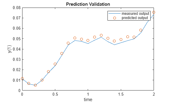
The predicted output closely matches the output in the validation data set. The result indicates that you can proceed to the next step of the data-driven MPC design.

Specify bounds and weights

As in classical MPC design, use the ManipulatedVariables and OutputVariables properties to define the bounds for the input and output variables.

ddobj.ManipulatedVariables.Min = -5;
ddobj.ManipulatedVariables.Max = 5;
ddobj.ManipulatedVariables.RateMin = -0.5;
ddobj.ManipulatedVariables.RateMax = 0.5;

Use the Weights property to define the weights of the quadratic cost function. For this example, set the first weight element in Weights.OutputVariables, which corresponds to the current output y[k], to 0. This setting is useful to later compare the solution to classical MPC, since for classical MPC the prediction starts at time k+1.

ddobj.Weights.OutputVariables = [0;ones(20,1)];

Weights.HankelVariables is a scalar weight that penalizes large values in decision variables, and thus, helps mitigate the influence of data errors and nonlinearities. Setting it to 0 effectively removes regularization and is not recommended. Conversely, setting it to large values can excessively distort the intended cost function of your controller.

ddobj.Weights.HankelVariables = 1e-4;

Weights.SlackPastU and Weights.SlackPastY are scalar weights that soften the equality constraints that are applied to past trajectories. These two weights make data-driven MPC more robust to measurement noises. Setting one or both values to inf partially or fully disables constraint softening and can lead to an infeasible optimization problem.

ddobj.Weights.SlackPastU = 1e4;
ddobj.Weights.SlackPastY = 1e4;

Simulate Closed-Loop Response

You can use either mpcmove or sim to simulate data-driven MPC in closed-loop. The sim function simulates the MPC controller against its own internal plant model. For this example, use mpcmove instead to simulate the controller against the true plant.

Define the DataDrivenMPCState object stateobj. The initial condition defaults to 0.

stateobj = DataDrivenMPCState(ddobj);       

Define a step reference signal.

ref = 1;                                
yref = repmat(ref,ddobj.FutureSteps,1);

Define the number of simulation steps.

simulationSteps = 51;                   

Define storage variables for the plant input and output.

yHistory = zeros(simulationSteps,1);
uHistory = zeros(simulationSteps,1);

Execute the simulation loop.

u = u0;
y = y0;
x = x0;
for ct=1:simulationSteps
    % Compute the optimal control action u[k].
    u = mpcmove(ddobj,stateobj,u,y,yref);
    % Store u[k].
    uHistory(ct) = u;
    % Simulate true plant from k to k+1 using lsim.
    [y,~,x] = lsim(sys,[u u],[0 Ts],x);
    % Extract x[k+1].
    x = x(2,:)';
    % Extract y[k].
    y = y(1);
    % Store y[k].
    yHistory(ct) = y;                       
end

Plot the response.

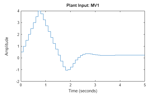
figure
subplot(2,1,1)
stairs((0:simulationSteps-1)*Ts,uHistory);
title('Plant Input: MV1');
xlabel('Time (seconds)');ylabel('Amplitude')
subplot(2,1,2);
stairs((0:simulationSteps-1)*Ts,yHistory);
title('Plant Output: OV1');
xlabel('Time (seconds)');ylabel('Amplitude')

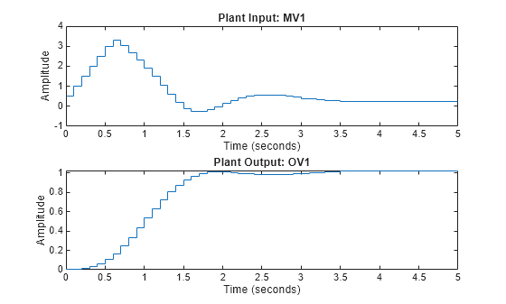
The data-driven MPC controller successfully drives the plant to follow the reference.

Simulation with Data-Driven MPC Block in Simulink

The Data-Driven MPC block implements the designed data-driven MPC controller in Simulink. Open the example model and run the simulation.

open_system('DDMPCwithMSD');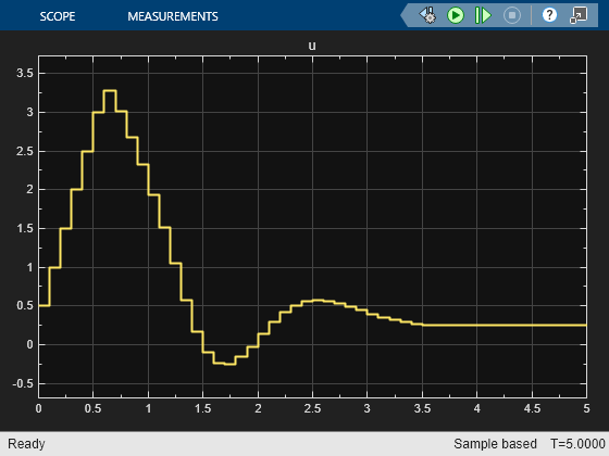
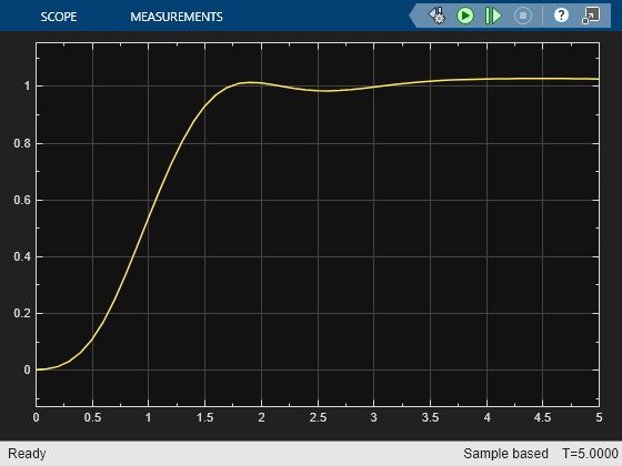
sim('DDMPCwithMSD');

The closed loop response is identical to the simulation result in MATLAB.

Compare Results with Classical MPC Design Using Identified Plant Model

Classical linear MPC design requires a linear plant model for prediction. The linear model can be derived from first principles or identified from experiment data obtained at a specific operating point. In this section, you compare the data-driven MPC design with a classical MPC design based on system identification.

First, use the ssest (System Identification Toolbox) function to identify the linear system sysEst, based on an open-loop experiment data set carried out with the true plant sys at the initial condition. If ssest is not available, set sysEst to a predefined variable.

if mpcchecktoolboxinstalled('ident')

    % Construct iddata object.
    data = iddata(dataY, dataU, Ts);

    % Identify state space system.
    idsys = ssest(data, nx);

    % Convert system into state space object.
    sysEst = ss(idsys);      

else

    % Assign sysEst variable.
    sysEst = ss([0.146 0.5629 -0.0612 -0.4745; ...
        -1.042 -1.848 0.513 -3.283; ...
        -0.6616 -4.784 -0.7897 22.43; ...
        1.758 7.014 -5.556 -44.97], ...
        [0.1259; -2.356; -0.9029; 0.2737], ...
        [-0.9966 -0.06868 0.01801 0.02413], ...
        0);      

end

Visualize Bode plots of both the true plant sys and the estimated plant sysEst.

figure;
bode(sys,sysEst);
legend('truth','identified');

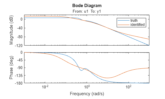
Comparing the Bode plots indicates that the estimated plant has modeling errors especially at higher frequencies, as the plots do not perfectly overlap.

Now, use the identified model sysEst to design a linear MPC controller. You compare the performance of this linear MPC controller to the data-driven MPC controller.

mpcobj = mpc(sysEst, Ts);

-->"PredictionHorizon" is empty. Assuming default 10.
-->"ControlHorizon" is empty. Assuming default 2.
-->"Weights.ManipulatedVariables" is empty. Assuming default 0.00000.
-->"Weights.ManipulatedVariablesRate" is empty. Assuming default 0.10000.
-->"Weights.OutputVariables" is empty. Assuming default 1.00000.

Set prediction time to 2 seconds.

mpcobj.PredictionHorizon = 20;

Set control horizon such that each control move across the prediction horizon is a free move.

mpcobj.ControlHorizon = 20;

Set external force F lower and upper bounds to -5 and 5, respectively.

mpcobj.MV.Min = -5;
mpcobj.MV.Max = 5;

Set input rate bounds so that F cannot decrease or increase more than 0.5 at each control interval.

mpcobj.MV.RateMin = -0.5;          
mpcobj.MV.RateMax = 0.5;

For simulation comparison, turn off the built-in disturbance observer in classical MPC because data-driven MPC does not have one.

setoutdist(mpcobj,'model',tf(0));   

Simulate the closed-loop response of the MPC controller (against the true plant) to a step reference change.

Create a simulation option object.

options = mpcsimopt;                    

Set up the true plant model.

options.Model = sys;                    

To simulate the closed loop system, use the sim command.

sim(mpcobj,simulationSteps,ref,options);

-->Converting model to discrete time.
-->"Model.Noise" is empty. Assuming white noise on each measured output.
-->Converting model to discrete time.

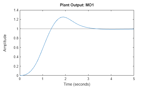
Note that, since the built-in disturbance rejection function is not used in the classical MPC, a nonzero steady-state offset is expected due to modeling errors.

Compared to the classical MPC design, the data-driven controller stabilizes the plant faster, with no overshoot, and using less control effort.