Create Binned Scatter Plot from Latitude and Longitude Data

Since R2026a

This example shows how to create a binned scatter plot from points in latitude and longitude coordinates. A binned scatter plot is a type of heatmap that partitions the points into rectangular bins and displays the number of points in each bin using colors along a gradient. Other types of heatmaps that you can create on maps include:

• Choropleth maps, which display the values of numeric attributes within polygons. For an example, see Create Choropleth Map from Table Data.

• Density plots, which display the relative distribution of points in latitude and longitude coordinates. For an example, see Visualize Density Using Geographic Density Plots.

• Pseudocolor raster plots, which display the values stored in a raster. For examples, see the geopcolor reference page.

For Cartesian axes, you can create a binned scatter plot by using the binscatter or histogram2 function. These functions automatically partition and display the points. For geographic axes and map axes, you must manually partition the data into bins by creating a referenced raster of bin counts. Then, you can display the raster of bin counts by using the geopcolor function.

This example creates a binned scatter plot from cyclone track data in latitude and longitude coordinates. The example involves these steps:

• Read the data into the workspace.

• Project the latitude and longitude coordinates to xy-coordinates.

• Partition the projected coordinates into bins.

• Create a raster reference object for the bins.

• Display the raster of bin counts on a map.

Read Data

Read scattered point data into the workspace as arrays of coordinates.

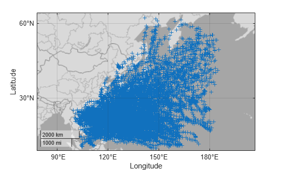
Load a table containing cyclone track data [1] into the workspace. The table includes the locations of over 200 cyclones, measured at six-hour intervals. Extract the latitude and longitude coordinates from the table.

load cycloneTracks.mat
lat = cycloneTracks.Latitude;
lon = cycloneTracks.Longitude;

Preview the data by displaying the latitude and longitude coordinates on a map.

figure
geobasemap darkwater
geoscatter(lat,lon,"+")

Project Coordinates

Prepare to partition the coordinates into bins by projecting the latitude and longitude coordinates to xy-coordinates. Working in xy-coordinates ensures that all the bins have the same dimensions in linear units. If you decide to work in latitude and longitude coordinates, then the bins will have the same dimensions in angular units but different dimensions in linear units. As a result, working with latitude and longitude coordinates can affect the appearance of the plot, especially for large or polar regions.

Create a projected coordinate reference system (CRS) object that is appropriate for the region by using the projcrs function. For this example, use the Asia South Lambert Conformal Conic projected CRS, which has the ESRI authority code 102030. If your data is already in xy-coordinates, then prepare to display the binned scatter plot by creating a projected CRS object for the coordinates.

proj = projcrs(102030,Authority="ESRI");

Project the latitude and longitude coordinates to xy-coordinates by using the projfwd function.

[x,y] = projfwd(proj,lat,lon);

Create Reference Object

Create a raster reference object for the projected coordinates by using the maprefcells function, the xy-limits of the raster, and a resolution that you specify. The maprefcells function creates a reference object for a regularly spaced raster of cells in projected coordinates, where each cell represents an area.

Calculate the xy-limits of the raster.

[xmin,xmax] = bounds(x,"all");
xlimits = [xmin xmax];

[ymin,ymax] = bounds(y,"all");
ylimits = [ymin ymax];

Specify the height and width of each cell in the raster. For this example, specify the height and width as approximately 1 degree by converting 1 degree to kilometers along a great circle on a sphere with a radius of 6371 kilometers. Then, to match the length unit of the CRS, convert the height and width from kilometers to meters.

cellhw = deg2km(1)*1000;

Create the reference object by using the maprefcells function. Specify the xy-limits and the height and width of each cell as inputs to the function. Then, specify the projected CRS of the reference object.

R = maprefcells(xlimits,ylimits,cellhw,cellhw);
R.ProjectedCRS = proj;

Partition Coordinates into Bins

Partition the coordinates into bins, where each bin represents one cell in the raster.

Define the bin edges in the x-dimension. Specify the leading edge of the first bin and the trailing edge of the last bin by querying the x-limits that are stored in the reference object. Note that the x-limits stored in the reference object can be different from the x-limits used to create the reference object, due to adjustments that the maprefcells function makes when creating the object. Then, specify the bin edges by incrementing from the leading edge of the first bin to the trailing edge of the last bin. Specify the increment using the width of each cell.

xStart = R.XWorldLimits(1);
xInc = R.CellExtentInWorldX;
xEnd = R.XWorldLimits(2);
xEdges = xStart:xInc:xEnd;

Define the bin edges in the y-dimension.

yStart = R.YWorldLimits(1);
yInc = R.CellExtentInWorldY;
yEnd = R.YWorldLimits(2);
yEdges = yStart:yInc:yEnd;

Determine the number of points within each bin by using the histcounts2 function. Specify the projected xy-coordinates, the bin edges in the x-dimension, and the bin edges in the y-dimension as inputs to the function.

N = histcounts2(x,y,xEdges,yEdges);

The histcounts2 function returns a matrix of bin counts, where each row corresponds to an x-value and each column corresponds to a y-value. Raster reference objects expect the opposite, where each row corresponds to a y-value and each column corresponds to an x-value. Reformat the matrix by calculating its transpose.

NT = N';

Verify that the transposed matrix of bin counts is compatible with the reference object by comparing the height and width of the transposed bin counts with the value stored in the RasterSize property of the reference object.

sz = size(NT);
isequal(sz,R.RasterSize)

ans = logical
   1

Create Binned Scatter Plot

Create the binned scatter plot by displaying the bin counts on a map.

Create a map that uses the Asia South Lambert Conformal Conic projected CRS.

figure
newmap(proj)

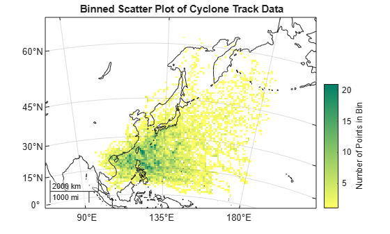
Display the bin counts by using the geopcolor function. Specify the transposed matrix of bin counts and the reference object as inputs to the function. Avoid displaying the empty bins by specifying the MissingDataIndicator argument as 0.

hold on
geopcolor(NT,R,MissingDataIndicator=0)

Provide geographic context for the plot by displaying a subset of world land areas.

land = readgeotable("landareas.shp");
subland = land([1:3,5:end],:);
geoplot(subland,FaceColor="none")

Center the plot by changing the geographic limits of the map.

geolimits([0 65],[90 190])

Add a labeled color bar, change the colormap, and add a title.

cb = colorbar;
cb.Label.String = "Number of Points in Bin";

cmap = flipud(summer);
colormap(cmap)

title("Binned Scatter Plot of Cyclone Track Data")

References

[1] This example uses modified RSMC Best Track Data from the Japan Meteorological Agency.