PointNet++ 深層学習を使用した航空 LiDAR のセマンティックセグメンテーション

この例では次を使用します。

この例では、航空 LiDAR データのセマンティックセグメンテーションを実行するために PointNet++ 深層学習ネットワークに学習させる方法を示します。

航空レーザースキャンシステムから取得される LiDAR データは、地形図作成、都市モデリング、バイオマス測定、災害管理などの用途に使用されます。このデータから意味のある情報を抽出するには、点群の各点に一意のクラスラベルを割り当てるセマンティックセグメンテーションのプロセスが必要になります。

この例では、セマンティックセグメンテーションを実行するために、Dayton Annotated Lidar Earth Scan (DALES) データセット [1] を使用して PointNet++ ネットワークに学習させます。このデータセットには、都市部、郊外、農村地域、および商業地域のシーンについて、ラベルが付けられた高密度の航空 LiDAR データが含まれています。データセットには、建物、自動車、トラック、ポール、電力線、フェンス、地面、植生の 8 つのクラスに対するセマンティックセグメンテーションラベルが用意されています。

DALES データの読み込み

DALES データセットには、40 個のシーンの航空 LiDAR データが含まれています。40 個のシーンのうち、29 個のシーンを学習に使用し、残りの 11 個のシーンをテストに使用します。データの各ピクセルにクラスラベルがあります。DALES の Web サイトの説明に従って、変数 dataFolder で指定したフォルダーにデータセットをダウンロードします。学習データとテストデータを格納するためのフォルダーを作成します。

dataFolder = fullfile(tempdir,'DALES');
trainDataFolder = fullfile(dataFolder,'dales_las','train');
testDataFolder = fullfile(dataFolder,'dales_las','test');

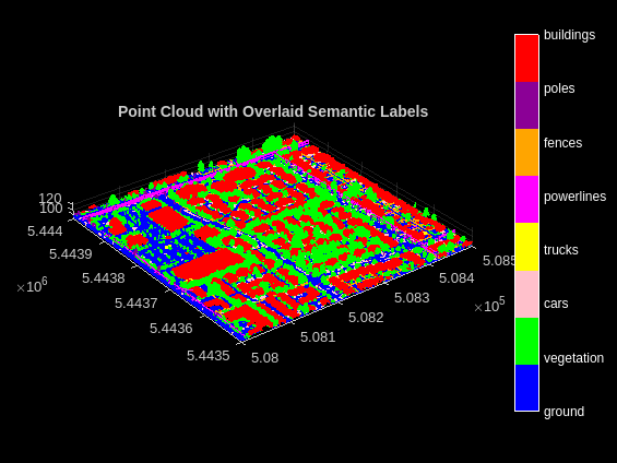
学習データから点群をプレビューします。

lasReader = lasFileReader(fullfile(trainDataFolder,'5080_54435.las'));
[pc,attr] = readPointCloud(lasReader,'Attributes','Classification');
labels = attr.Classification;

% Select only labeled data.
pc = select(pc,labels~=0);
labels = labels(labels~=0);
classNames = [
    "ground"
    "vegetation"
    "cars"
    "trucks"
    "powerlines"
    "fences"
    "poles"
    "buildings"
    ];
figure;
ax = pcshow(pc.Location,labels);
helperLabelColorbar(ax,classNames);
title("Point Cloud with Overlaid Semantic Labels");

データの前処理

DALES データセットの各点群は、地上 LiDAR 点群でカバーされる一般的な領域よりもはるかに大きい 500×500 メートルの領域をカバーします。効率的なメモリ処理のために、blockedPointCloudオブジェクトを使用して、オーバーラップしない小さなブロックに点群を分割します。

blockSize パラメーターを使用してブロックの寸法を定義します。データセット内の各点群のサイズは変化するため、ブロックの z 次元を Inf に設定して、z 軸に沿ってブロックが作成されないようにします。

blocksize = [51 51 Inf];

学習データのすべての点群ファイルを収集するためのmatlab.io.datastore.FileSetオブジェクトを作成します。

fs = matlab.io.datastore.FileSet(trainDataFolder);

Fileset オブジェクトを使用してblockedPointCloudオブジェクトを作成します。

bpc = blockedPointCloud(fs,blocksize);

メモ: 処理には時間がかかることがあります。このコードは、処理が完了するまで、MATLAB® の実行を一時停止します。

この例にサポートファイルとして添付されている補助関数 helperCalculateClassWeights を使用して、学習データセット内のすべてのクラスにおける点の分布を計算します。

numClasses = numel(classNames);
[weights,maxLabel,maxWeight] = helperCalculateClassWeights(fs,numClasses);

学習用のデータストアオブジェクトの作成

ネットワークの学習用に、ブロック化された点群 bpc を使用してblockedPointCloudDatastoreオブジェクトを作成します。

ldsTrain = blockedPointCloudDatastore(bpc,MinPoints=10);

1 からクラス数までのラベル ID を指定します。

labelIDs = 1 : numClasses;

点群をプレビューして表示します。

ptcld = preview(ldsTrain);
figure;
pcshow(ptcld.Location);
title("Cropped Point Cloud");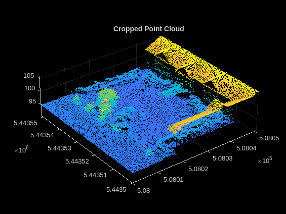

学習を高速化するために、ブロックごとの固定の点の数を設定します。

numPoints = 8192;

この例の終わりに定義されている関数 helperTransformToTrainData を使用して、ネットワークの入力層と互換性をもつようにデータを変換します。次の手順に従って変換を適用します。

点群と対応するラベルを抽出する。
点群とラベルを指定の数 numPoints にダウンサンプリングする。
点群を範囲 [0 1] に正規化する。
ネットワークの入力層と互換性をもつように点群と対応するラベルを変換する。

ldsTransformed = transform(ldsTrain,@(x,info) helperTransformToTrainData(x, ...
    numPoints,info,labelIDs,classNames),'IncludeInfo',true);
read(ldsTransformed)

ans=1×2 cell array
    {8192×3 double}    {8192×1 categorical}

PointNet++ モデルの定義

PointNet++ は、アンオーガナイズド LiDAR 点群のセマンティックセグメンテーションによく使用されるニューラルネットワークです。セマンティックセグメンテーションにより、3 次元点群の各点が自動車、トラック、地面、植生などのクラスラベルに関連付けられます。詳細については、PointNet++ 入門を参照してください。

関数 pointnetplusNetwork を使用して PointNet++ のアーキテクチャを定義します。

lgraph = pointnetplusNetwork(numPoints,3,numClasses);

DALES データセットのクラスの不平衡に対処するために、加重損失関数crossentropy (Deep Learning Toolbox)を使用します。これにより、重みの小さいクラスに属する点が誤って分類された場合に、さらに高いペナルティがネットワークに課されるようになります。

% Define the loss function.
lossfun = @(Y,T) mean(mean(sum(crossentropy(Y,T,weights,'WeightsFormat','UC','Reduction','none'),3),1),4);

学習オプションの指定

ネットワークの学習には Adam 最適化アルゴリズムを使用します。関数trainingOptions (Deep Learning Toolbox)を使用してハイパーパラメーターを指定します。

CPU または GPU を使用してネットワークに学習させます。GPU を使用するには、Parallel Computing Toolbox™、および CUDA® 対応の NVIDIA® GPU が必要です。詳細については、GPU 計算の要件 (Parallel Computing Toolbox)を参照してください。使用できる GPU があるかどうかを自動的に検出するには、executionEnvironment を "auto" に設定します。GPU がない場合、または学習で GPU を使用しない場合は、executionEnvironment を "cpu" に設定します。学習に GPU が使用されるようにするには、executionEnvironment を "gpu" に設定します。

executionEnvironment = "auto";
if canUseParallelPool
    dispatchInBackground = true;
else
    dispatchInBackground = false;
end

learningRate = 0.0005;
l2Regularization = 0.01;
numEpochs = 20;
miniBatchSize = 16;
learnRateDropFactor = 0.1;
learnRateDropPeriod = 10;
gradientDecayFactor = 0.9;
squaredGradientDecayFactor = 0.999;

options = trainingOptions('adam', ...
    'InitialLearnRate',learningRate, ...
    'L2Regularization',l2Regularization, ...
    'MaxEpochs',numEpochs, ...
    'MiniBatchSize',miniBatchSize, ...
    'LearnRateSchedule','piecewise', ...
    'LearnRateDropFactor',learnRateDropFactor, ...
    'LearnRateDropPeriod',learnRateDropPeriod, ...
    'GradientDecayFactor',gradientDecayFactor, ...
    'SquaredGradientDecayFactor',squaredGradientDecayFactor, ...
    'ExecutionEnvironment',executionEnvironment, ...
    'DispatchInBackground',dispatchInBackground, ...
    'Plots','training-progress');

メモ: 学習時にメモリ使用量を制御できるように miniBatchSize の値は小さくしてください。

モデルの学習

ネットワークに学習させるには、doTraining 引数を true に設定します。そうでない場合は、事前学習済みのネットワークを読み込みます。ネットワークの学習には CPU または GPU を使用できます。GPU を使用するには、Parallel Computing Toolbox™、および CUDA® 対応の NVIDIA® GPU が必要です。詳細については、GPU 計算の要件 (Parallel Computing Toolbox)を参照してください。

doTraining = false;
if doTraining
    % Train the network on the ldsTransformed datastore using 
    % the trainnet function.
    [net,info] = trainnet(ldsTransformed,net,lossfun,options);
else
    % Load the pretrained network.
    load('pointnetplusNetworkTrained','net');
end

航空点群のセグメント化

テスト用の点群でセグメンテーションを実行するには、まずblockedPointCloudオブジェクトを作成し、次にblockedPointCloudDatastoreオブジェクトを作成します。

学習データで使用したのと同様の変換をテストデータに適用します。

点群と対応するラベルを抽出する。
点群を指定の数 numPoints にダウンサンプリングする。
点群を範囲 [0 1] に正規化する。
ネットワークの入力層と互換性をもつように点群を変換する。

tbpc = blockedPointCloud(fullfile(testDataFolder,'5080_54470.las'),blocksize);
tbpcds = blockedPointCloudDatastore(tbpc);

ダウンサンプリングされた点群から高密度点群の各点に対する最近傍点を見つけ、内挿を効率的に実行できるように、numNearestNeighbors と radius を定義します。

numNearestNeighbors = 20;
radius = 0.05;

予測用に空のプレースホルダーを初期化します。

labelsDensePred = [];

このテスト用の点群で推定を実行して、予測ラベルを計算します。予測ラベルを内挿して、高密度点群の予測ラベルを取得します。関数pcsemanticsegを使用して、オーバーラップしないすべてのブロックで処理を反復してラベルを予測します。

while hasdata(tbpcds)

    % Read the block along with block information.
    ptCloudDense = read(tbpcds);

    % Use the helperDownsamplePoints function, attached to this example as a
    % supporting file, to extract a downsampled point cloud from the
    % dense point cloud.
    ptCloudSparse = helperDownsamplePoints(ptCloudDense{1},[],numPoints);
                       
    % Use the helperNormalizePointCloud function, attached to this example as
    % a supporting file, to normalize the point cloud between 0 and 1.
    ptCloudSparseNormalized = helperNormalizePointCloud(ptCloudSparse);
    ptCloudDenseNormalized = helperNormalizePointCloud(ptCloudDense{1});
    
    % Use the helperTransformToTestData function, defined at the end of this
    % example, to convert the point cloud to a cell array and to permute the
    % dimensions of the point cloud to make it compatible with the input layer
    % of the network.
    ptCloudSparseForPrediction = helperTransformToTestData(ptCloudSparseNormalized);
    
    % Get the output predictions.
    labelsSparsePred = predict(net,ptCloudSparseForPrediction{1,1});
    [~,labelsSparsePred] = max(labelsSparsePred,[],3);
    
    % Use the helperInterpolate function, attached to this example as a
    % supporting file, to calculate labels for the dense point cloud,
    % using the sparse point cloud and labels predicted on the sparse point cloud.
    interpolatedLabels = helperInterpolate(ptCloudDenseNormalized, ...
        ptCloudSparseNormalized,labelsSparsePred,numNearestNeighbors, ...
        radius,maxLabel,numClasses);  
    
    % Concatenate the predicted labels from the blocks.
    labelsDensePred = vertcat(labelsDensePred,interpolatedLabels);
end

Starting parallel pool (parpool) using the 'Processes' profile ...
Connected to parallel pool with 32 workers.

見やすいように、点群データから推定されたブロックのみを表示します。

figure;
ax = pcshow(ptCloudDense{1}.Location,interpolatedLabels);
axis off;
helperLabelColorbar(ax,classNames);
title("Point Cloud Overlaid with Detected Semantic Labels");

ネットワークの評価

テストデータで評価を実行するには、テスト点群からラベルを取得します。テストデータのラベルは、前の手順で既に予測されています。したがって、オーバーラップしていない点群のブロックを反復してグラウンドトゥルースラベルを抽出します。

ターゲットラベルのプレースホルダーを初期化します。

labelsDenseTarget = [];

ブロックの点群データストアをループ処理してグラウンドトゥルースラベルを取得します。

reset(tbpcds);

while hasdata(tbpcds)    
    % Read the block along with block information.
    [~,infoDense] = read(tbpcds);

    % Extract the labels from the block information.
    labelsDense = infoDense.PointAttributes.Classification;
    
    % Concatenate the target labels from the blocks.
    labelsDenseTarget = vertcat(labelsDenseTarget,labelsDense);
end

関数evaluateSemanticSegmentationを使用して、テストセットの結果からセマンティックセグメンテーションのメトリクスを計算します。ターゲットラベルと予測ラベルは、前に計算したものが変数 labelsDensePred と labelsDenseTarget にそれぞれ格納されています。

confusionMatrix = segmentationConfusionMatrix(double(labelsDensePred), ...
    double(labelsDenseTarget),'Classes',1:numClasses);
metrics = evaluateSemanticSegmentation({confusionMatrix},classNames,'Verbose',false);

Intersection-over-Union (IoU) メトリクスを使用してクラスごとのオーバーラップ量を測定できます。

関数evaluateSemanticSegmentationは、データセット全体、個々のクラス、および各テストイメージについてのメトリクスを返します。データセットレベルのメトリクスを確認するには、metrics.DataSetMetrics プロパティを使用します。

metrics.DataSetMetrics

ans=1×4 table
    GlobalAccuracy    MeanAccuracy    MeanIoU    WeightedIoU
    ______________    ____________    _______    ___________

       0.93648          0.66492       0.5344       0.89048

データセットメトリクスは、ネットワークパフォーマンスのおおまかな概要を提供します。全体のパフォーマンスに対する各クラスの影響を確認するには、metrics.ClassMetrics プロパティを使用して各クラスのメトリクスを検査します。

metrics.ClassMetrics

ans=8×2 table
                  Accuracy      IoU   
                  ________    ________

    ground        0.99254        0.943
    vegetation    0.85796      0.83182
    cars          0.57798      0.40791
    trucks        0.15883     0.056435
    powerlines    0.75769      0.67357
    fences        0.50396      0.24061
    poles         0.53049      0.22384
    buildings     0.93989      0.89801

全体的なネットワークパフォーマンスは良好ですが、Trucks などの一部のクラスのクラスメトリクスから、パフォーマンスを向上させるためにより多くの学習データが必要であることがわかります。

サポート関数

関数 helperLabelColorbar は、現在の軸にカラーバーを追加します。カラーバーは、クラス名を色で表示するように書式設定されています。

function helperLabelColorbar(ax,classNames)
% Colormap for the original classes.
cmap = [[0 0 255];
    [0 255 0];
    [255 192 203];
    [255 255 0];
    [255 0 255];
    [255 165 0];
    [139 0 150];
    [255 0 0]];
cmap = cmap./255;
cmap = cmap(1:numel(classNames),:);
colormap(ax,cmap);

% Add colorbar to current figure.
c = colorbar(ax);
c.Color = 'w';

% Center tick labels and use class names for tick marks.
numClasses = size(classNames,1);
c.Ticks = 1:1:numClasses;
c.TickLabels = classNames;

% Remove tick mark.
c.TickLength = 0;
end

関数 helperTransformToTrainData は、入力データに対して次の一連の変換を実行します。

点群と対応するラベルを抽出する。
点群とラベルを指定の数 numPoints にダウンサンプリングする。
点群を範囲 [0 1] に正規化する。
ネットワークの入力層と互換性をもつように点群と対応するラベルを変換する。

function [cellout,dataout] = helperTransformToTrainData(data,numPoints,info,...
    labelIDs,classNames)
if ~iscell(data)
    data = {data};
end
numObservations = size(data,1);
cellout = cell(numObservations,2);
dataout = cell(numObservations,2);
for i = 1:numObservations 
    classification = info.PointAttributes(i).Classification;

    % Remove labels with zero value.
    pc = data{i,1};
    pc = select(pc,(classification ~= 0));
    classification = classification(classification ~= 0);

    % Use the helperDownsamplePoints function, attached to this example as a
    % supporting file, to extract a downsampled point cloud and its labels
    % from the dense point cloud.
    [ptCloudOut,labelsOut] = helperDownsamplePoints(pc, ...
    classification,numPoints);

    % Make the spatial extent of the dense point cloud and the sparse point
    % cloud same.
    limits = [ptCloudOut.XLimits;ptCloudOut.YLimits;...
                    ptCloudOut.ZLimits];
    ptCloudSparseLocation = ptCloudOut.Location;
    ptCloudSparseLocation(1:2,:) = limits(:,1:2)';
    ptCloudSparseUpdated = pointCloud(ptCloudSparseLocation, ...
        'Intensity',ptCloudOut.Intensity, ...
        'Color',ptCloudOut.Color, ...
        'Normal',ptCloudOut.Normal);

    % Use the helperNormalizePointCloud function, attached to this example as
    % a supporting file, to normalize the point cloud between 0 and 1.    
    ptCloudOutSparse = helperNormalizePointCloud( ...
        ptCloudSparseUpdated);
    cellout{i,1} = ptCloudOutSparse.Location;

    % Permuted output.
    cellout{i,2} = permute(categorical(labelsOut,labelIDs,classNames),[1 3 2]);

    % General output.
    dataout{i,1} = ptCloudOutSparse;
    dataout{i,2} = labelsOut;
end
end

関数 helperTransformToTestData は、ネットワークの入力層と互換性をもつように点群を cell 配列に変換して点群の次元を並べ替えます。

function data = helperTransformToTestData(data)
if ~iscell(data)
    data = {data};
end
numObservations = size(data,1);
for i = 1:numObservations
    tmp = data{i,1}.Location;
    data{i,1} = tmp;
end
end

参考文献

[1] Varney, Nina, Vijayan K. Asari, and Quinn Graehling. "DALES: A Large-Scale Aerial LiDAR dataset for Semantic Segmentation." ArXiv:2004.11985 [Cs, Stat], April 14, 2020. https://arxiv.org/abs/2004.11985.

[2] Qi, Charles R., Li Yi, Hao Su, and Leonidas J. Guibas. "PointNet++: Deep Hierarchical Feature Learning on Point Sets in a Metric Space." ArXiv:1706.02413 [Cs], June 7, 2017. https://arxiv.org/abs/1706.02413.

PointNet++ 深層学習を使用した航空 LiDAR のセマンティック セグメンテーション