Detect and Count Cell Nuclei in Whole Slide Images
This example shows how to detect and count cell nuclei in whole slide images (WSIs) of tissue stained using hematoxylin and eosin (H&E).
Cell counting is an important step in most digital pathology workflows. The number and distribution of cells in a tissue sample can be a biomarker of cancer or other diseases. Digital pathology uses digital images of microscopy slides, or whole slide images (WSIs), for clinical diagnosis or research. To capture tissue- and cellular-level detail, WSIs have high resolutions and can have sizes on the order of 200,000-by-100,000 pixels. To facilitate efficient display, navigation, and processing of WSIs, the best practice is to store them in a multiresolution format. In MATLAB®, you can use blocked images to work with WSIs without loading the full image into core memory.
This example outlines an approach to cell nuclei detection and counting using blocked images. To ensure that the detection algorithm counts cells on block borders only once, this blocked image approach uses overlapping borders. Although this example uses a simple cell detection algorithm, you can use the blocked image approach to create more sophisticated algorithms and implement deep learning techniques.
The Medical Imaging Toolbox™ Interface for Cellpose Library support package provides functionality and pretrained models for segmenting cells and cell nuclei. For a version of this example that more accurately segments nuclei using cellpose, see Detect Nuclei in Large Whole Slide Images Using Cellpose (Medical Imaging Toolbox).
Download Sample Image from Camelyon17 Data Set
This example uses one WSI from the Camelyon17 challenge data set. This data set contains 400 whole-slide images (WSIs) of lymph nodes, stored as multiresolution TIF files that are too large to be loaded into memory.
Run this code to download the patient_000_node_1.zip file from the MathWorks® website, then unzip the file. The size of the data file is approximately 1.32 GB.
zipFile = matlab.internal.examples.downloadSupportFile( ...
    "image","data/camelyon17/patient_000_node_1.zip");
filepath = fileparts(zipFile);
unzip(zipFile,filepath)
Specify the filename of the TIF file.
fileName = fullfile(filepath,"patient_000_node_1.tif");Create and Preprocess Blocked Image
Create a blockedImage object from the sample image. This image has nine resolution levels. The finest resolution level, which is the first level, has a size of 197226-by-96651 pixels. The coarsest resolution level, which is the last level, has a size of 770-by-377 pixels and easily fits in memory.
bim = blockedImage(fileName);
disp(bim.NumLevels)
9
disp(bim.Size)
      197226       96651           3
       98613       48325           3
       49306       24162           3
       24653       12081           3
       12326        6040           3
        6163        3020           3
        3081        1510           3
        1540         755           3
         770         377           3
Adjust Spatial Extents of Each Level
The TIF image metadata contains information about the world coordinates. The exact format of the metadata varies across different sources. The file in this example stores the mapping between pixel subscripts and world coordinates using the XResolution, YResolution, and ResolutionUnit fields. The TIFF standard indicates that XResolution and YResolution are the number of pixels per ResolutionUnit in the corresponding directions.
fileInfo = imfinfo(bim.Source);
info = table((1:9)',[fileInfo.XResolution]',[fileInfo.YResolution]',{fileInfo.ResolutionUnit}', ...
    VariableNames=["Level","XResolution","YResolution","ResolutionUnit"]);
disp(info)
Level XResolution YResolution ResolutionUnit
_____ ___________ ___________ ______________
1 41136 41136 {'Centimeter'}
2 20568 20568 {'Centimeter'}
3 10284 10284 {'Centimeter'}
4 5142.1 5142.1 {'Centimeter'}
5 2571 2571 {'Centimeter'}
6 1285.5 1285.5 {'Centimeter'}
7 642.76 642.76 {'Centimeter'}
8 321.38 321.38 {'Centimeter'}
9 160.69 160.69 {'Centimeter'}
Calculate the size of a single pixel, or the pixel extent, in world coordinates at the finest resolution level. The pixel extent is identical in the x and the y directions because the values of XResolution and YResolution are equal. Then, calculate the corresponding full image size in world coordinates.
level = 1;
pixelExtentInWorld = 1/fileInfo(level).XResolution;
imageSizeInWorld = bim.Size(level,1:2)*pixelExtentInWorld;
Adjust the spatial extents of each level such that the levels cover the same physical area in the real world. To ensure that subscripts map to pixel centers, offset the starting coordinate and the ending coordinate by a half pixel.
bim.WorldStart = [pixelExtentInWorld/2 pixelExtentInWorld/2 0.5];
bim.WorldEnd = bim.WorldStart + [imageSizeInWorld 3];
Display the image using the imageshow function.
img = imageshow(bim);
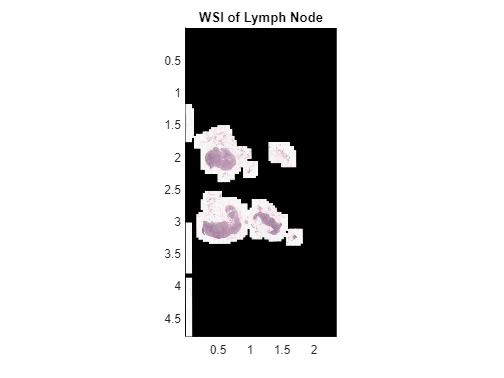
img.Parent.Title="WSI of Lymph Node";Develop Basic Nuclei Detection Algorithm
This example develops the nuclei detection algorithm using a representative region of interest (ROI), then applies the algorithm on all regions of the image that contain tissue.
Zoom in the image and identify the ROI.
xRegion = [0.53 0.55];
yRegion = [2.064 2.08];
Convert the world coordinates of the ROI to pixel subscripts. Then, extract the ROI data at the finest resolution level using the getRegion function.
subStart = world2sub(bim,[yRegion(1) xRegion(1)]);
subEnd   = world2sub(bim,[yRegion(2) xRegion(2)]);
imRegion = getRegion(bim,subStart,subEnd,Level=1);
hbim = imageshow(imRegion);
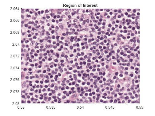
hbim.Parent.Title = "Region of Interest";Detect Nuclei Using Color Thresholding
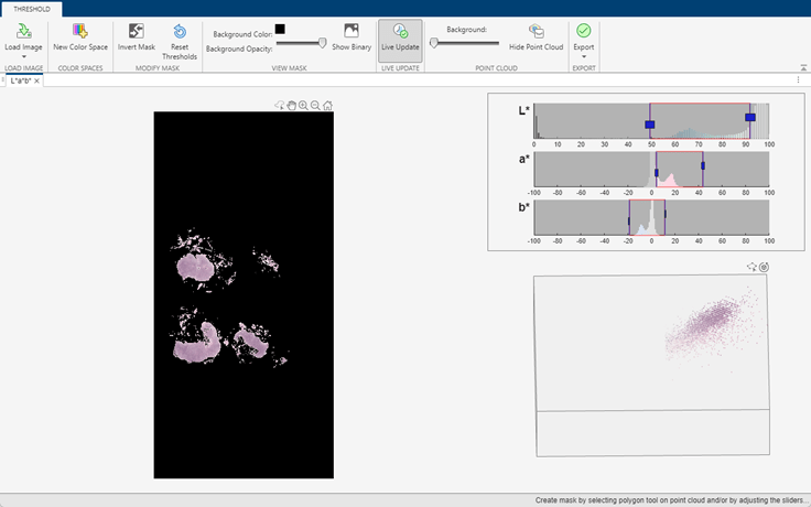
The nuclei have a distinct stain color that enables segmentation using color thresholding. This example provides a helper function, createNucleiMask, that segments nuclei using color thresholding in the RGB color space. The thresholds have been selected, and the code for the helper function has been generated, using the colorThresholder app. The helper function is attached to the example as a supporting file.
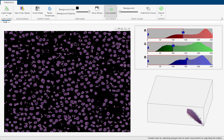
If you want to segment the nuclei regions using a different color space or select different thresholds, use the colorThresholder app. Open the app and load the image using this command:
colorThresholder(imRegion)
After you select a set of thresholds in the color space of your choice, generate the segmentation function by selecting Export from the toolstrip and then selecting Export Function. Save the generated function as createNucleiMask.m.
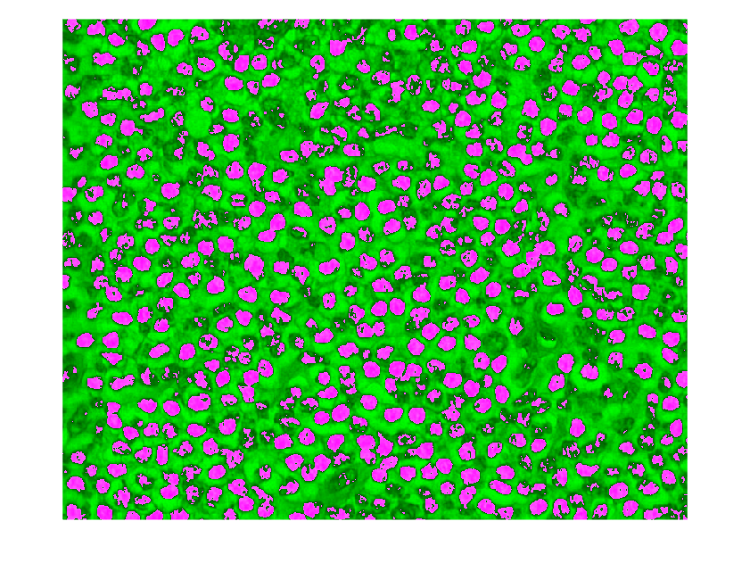
Apply the segmentation to the ROI, and display the mask over the ROI as a falsecolor composite image.
nucleiMask = createNucleiMask(imRegion);
hbim = imfuse(imRegion,nucleiMask);
imageshow(hbim);
Select Nuclei Using Image Region Properties
Explore properties of the regions in the mask using the imageRegionAnalyzer app. Open the app by using this command:
imageRegionAnalyzer(nucleiMask)
Clean up regions with holes inside the nuclei by selecting Fill Holes on the toolstrip. Display the Area and EquivDiameter properties using the Choose Properties dropdown on the toolstrip.
Sort the regions by area. Regions with the largest areas typically correspond to overlapping nuclei. Because your goal is to segment single cells, you can ignore the largest regions at the expense of potentially underestimating the total number of nuclei.
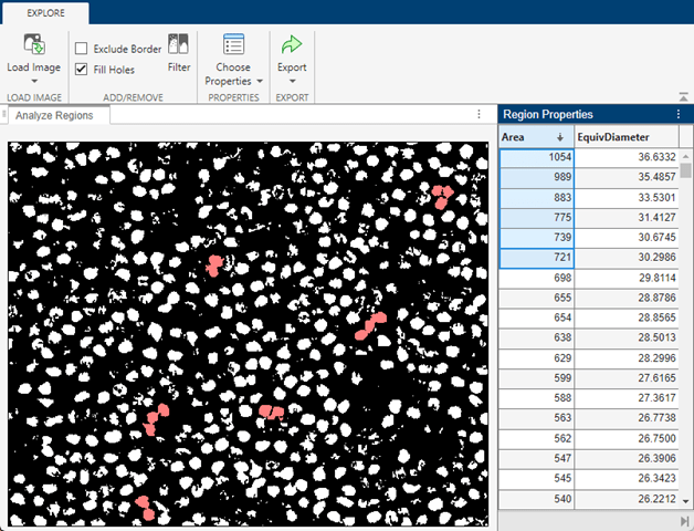
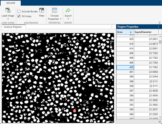
Scroll down the list until you find the largest region that corresponds to a single nucleus. Specify maxArea as the area of this region. Specify equivDiameter as the value of the EquivDiameter property for this region. Calculate the equivalent radius of the region as half the value of equivDiameter.
maxArea = 405;
equivDiameter = 22.7082;
equivRadius = round(equivDiameter/2);
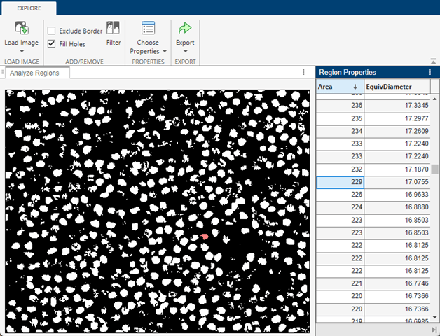
Regions with very small area typically correspond to partial nuclei. Continue scrolling until you find the smallest region that corresponds to a whole nucleus. Set minArea as the area of this region. Because your goal is to segment whole cells, you can ignore regions with areas smaller than minArea.
minArea = 229;
Filter the image so it contains only the regions with areas between minArea and maxArea. From the toolstrip, select Filter. The binary image updates in real time to reflect the current filtering parameters.
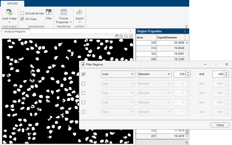
You can optionally change the range of areas or add additional region filtering constraints. For example, you can require that nuclei be approximately round by excluding regions with large perimeters. Specify the filter parameters in the Filter Regions dialog box.
This example provides a helper function, calculateNucleiProperties, that calculates the area and centroid of regions within the range of areas [229, 405]. The code for the helper function has been generated using the imageRegionAnalyzer app. The helper function is attached to the example as a supporting file.
If you specify different filtering constraints, then you must generate a new filtering function by selecting Export from the toolstrip and then selecting Export Function. Save the generated function as calculateNucleiProperties.m. After you generate the function, you must open the function and edit the last line of code so that the function returns the region centroids. Add 'Centroid' to the cell array of properties measured by the regionprops function. For example:
properties = regionprops(BW_out,{"Centroid","Area","Perimeter"});
Calculate the centroids for each likely detection by using the calculateNucleiProperties helper function. Overlay the centroids as yellow points over the ROI.
[~,stats] = calculateNucleiProperties(nucleiMask);
centroidCoords = vertcat(stats.Centroid);
hbim = imageshow(imRegion);
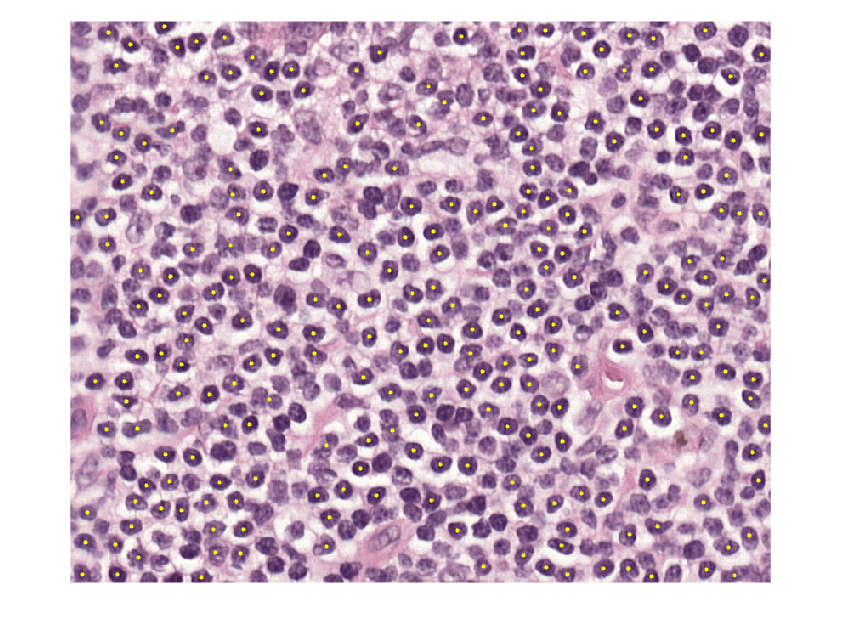
for ind = 1:length(centroidCoords)
    uidraw(hbim.Parent,"point",Position=[centroidCoords(ind,1),centroidCoords(ind,2)],Color="y",Label="",Interactions="none");
end
Apply Nuclei Detection Algorithm
To process WSI data efficiently at fine resolution levels, apply the nuclei detection algorithm on blocks consisting of tissue and ignore blocks without tissue. You can identify blocks with tissue using a coarse tissue mask. For more information, see Process Blocked Images Efficiently Using Mask.
Create Tissue Mask
The tissue is brighter than the background, which enables segmentation using color thresholding. This example provides a helper function, createTissueMask, that segments tissue using color thresholding in the L*a*b* color space. The thresholds have been selected, and the code for the helper function has been generated, using the colorThresholder app. The helper function is attached to the example as a supporting file.
If you want to segment the tissue using a different color space or select different thresholds, use the colorThresholder app. Open a low-resolution version of the image in the app using these commands:
imCoarse = gather(bim);
colorThresholder(imCoarse)
After you select a set of thresholds, generate the segmentation function by selecting Export from the toolstrip and then selecting Export Function. Save the generated function as createTissueMask.m.
Create a mask of the regions of interest that contain tissue by using the apply function. In this code, the apply function runs the createTissueMask function on each block of the original blocked image bim and assembles the tissue masks into a single blockedImage with the correct world coordinates. This example creates the mask at the seventh resolution level, which fits in memory and follows the contours of the tissue better than a mask at the coarsest resolution level.
maskLevel = 7;
tissueMask = apply(bim,@(bs)createTissueMask(bs.Data),Level=maskLevel);
Overlay the mask on the original WSI image using the imageshow function.
hbim = imageshow(bim,OverlayData=tissueMask,OverlayAlphamap=[0.3 0],OverlayDisplayRangeMode="data-range",OverlayColormap=[0.5 1 0.5]);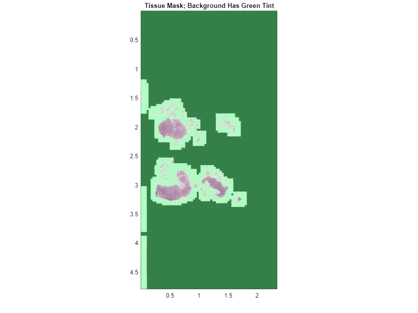
hbim.Parent.Title ="Tissue Mask; Background Has Green Tint";Select Blocks with Tissue
Select the set of blocks on which to run the nuclei detection algorithm by using the selectBlockLocations function. Include only blocks that have at least one pixel inside the mask by specifying the InclusionThreshold name-value argument as 0. Specify a large block size to perform the nuclei detection more efficiently. The upper limit of the block size depends on the amount of system RAM. If you perform the detection using parallel processing, you may need to reduce the block size.
blockSize = [2048 2048 3];
bls = selectBlockLocations(bim,BlockSize=blockSize, ...
    Masks=tissueMask,InclusionThreshold=0,Levels=1);
Apply Algorithm on Blocks with Tissue
Perform the nuclei detection on the selected blocks using the apply function. In this code, the apply function runs the countNuclei helper function (defined at the end of the example) on each block of the blocked image bim and returns a structure with information about the area and centroid of each nucleus in the block. To ensure the function detects and counts nuclei on the edges of a block only once, add a border size equal to the equivalent radius value of the largest nucleus region. To accelerate the processing time, process the blocks in parallel.
if(exist("bndetections","dir"))
    rmdir("bndetections","s")
end
bndetections = apply(bim,@(bs)countNuclei(bs), ...
    BlockLocationSet=bls,BorderSize=[equivRadius equivRadius], ...
    Adapter=images.blocked.MATBlocks,OutputLocation="bndetections", ...
    UseParallel=true);
Starting parallel pool (parpool) using the 'Processes' profile ...
12-Nov-2025 16:04:21: Job Queued. Waiting for parallel pool job with ID 1 to start ...
12-Nov-2025 16:05:23: Job Queued. Waiting for parallel pool job with ID 1 to start ...
12-Nov-2025 16:06:24: Job Queued. Waiting for parallel pool job with ID 1 to start ...
Connected to parallel pool with 8 workers.
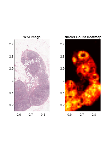
Display Heatmap of Detected Nuclei
Create a heatmap that shows the distribution of detected nuclei across the tissue sample. Each pixel in the heatmap contains the count of detected nuclei in a square of size 0.01-by-0.01 square centimeters in world coordinates.
Determine the number of pixels that this real world area contains:
numPixelsInSquare = world2sub(bim,[0.01 0.01]);
Calculate the size of the heatmap, in pixels, at the finest level. Then initialize a heatmap consisting of all zeros.
bimSize = bim.Size(1,1:2);
heatMapSize = round(bimSize./numPixelsInSquare);
heatMap = zeros(heatMapSize);
Load the blocked image of detected nuclei into memory. Get the list of the (row, column) pixel indices of the centroids of all detected nuclei.
ndetections = gather(bndetections);
centroidsPixelIndices = vertcat(ndetections.ncentroidsRC);
Map the nuclei centroid coordinates to pixels in the heatmap. First, normalize the (row, column) centroid indices relative to the size of the blocked image, in pixels. Then, multiply the normalized coordinates by the size of the heatmap to yield the (row, column) pixel indices of the centroids in the heatmap.
centroidsRelative = centroidsPixelIndices./bimSize;
centroidsInHeatmap = ceil(centroidsRelative.*heatMapSize);
Loop through the nuclei and, for each nucleus, increment the value of the corresponding heatmap pixel by one.
for ind = 1:length(centroidsInHeatmap)
    r = centroidsInHeatmap(ind,1);
    c = centroidsInHeatmap(ind,2);
    heatMap(r,c) = heatMap(r,c)+1;
end
Display the heatmap.
maxCount = max(heatMap,[],"all");
h = imageshow(heatMap,DisplayRangeMode="data-range",Colormap=hot(maxCount));
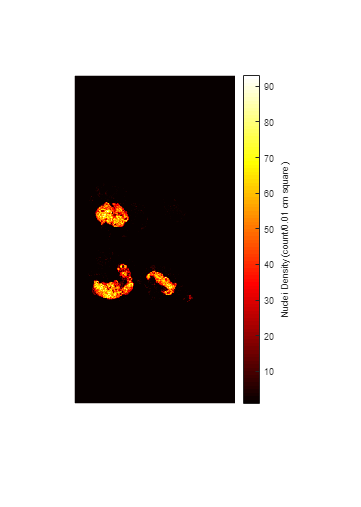
h.Parent.Title = "Nuclei Density (count/0.01 cm square)";Convert the heatmap into a blocked image with the correct world coordinates.
bHeatmap = blockedImage(heatMap, ...
    WorldStart=bim.WorldStart(1,1:2),WorldEnd=bim.WorldEnd(1,1:2));
Display the original WSI data next to the heatmap.
fig = uifigure;
g = uigridlayout(fig,ColumnWidth={"1x","1x"},RowHeight={"1x"});
viewer1 = viewer2d(g,ScaleBar="off");
viewer2 = viewer2d(g,ScaleBar="off");

viewer1.Layout.Row = 1;
viewer1.Layout.Column = 1;
viewer1.Title = "WSI Image";
viewer2.Layout.Row = 1;
viewer2.Layout.Column = 2;
viewer2.Title = "Nuclei Count Heatmap";

imageshow(bim,Parent=viewer1);

imageshow(bHeatmap,Parent=viewer2,DisplayRangeMode="data-range",Colormap=hot(maxCount));
Link the viewers of the two images to enable comparison and zoom in on an interesting region.
linkviewers([viewer1 viewer2]);
Inspect the detected nuclei across the entire WSI using the helper function exploreNucleiDetectionResults, which is attached to the example as a supporting file. The helper function displays the WSI with a draggable overview rectangle (shown in blue) next to a detail view of the portion of the image within the overview rectangle. You can move and resize the overview window interactively, and the detail view updates to display the new selected region and its centroids.
roi = [0.62333 2.0725 0.005 0.005];
h = exploreNucleiDetectionResults(bim,bndetections,roi);
Warning: Displaying large numbers of interactive annotations may impact performance. Consider removing unused or inessential annotations.

Supporting Function
The countNuclei helper function performs these operations to count nuclei within a block of blocked image data:
Create a binary mask of potential nuclei based on a color threshold, using the
createNucleiMaskhelper function. This function has been generated using thecolorThresholderapp and is attached to the example as a supporting file.Select individual nuclei within the binary mask based on region properties, and return the measured area and centroid of each nucleus, using the
calculateNucleiPropertieshelper function. This function has been generated using theimageRegionAnalyzerapp and is attached to the example as a supporting file.Create a structure containing the (row, column) coordinates of the top-left and bottom-right corners of the block, and the area and centroid measurements of nuclei within the block. Omit nuclei whose centroids are near the border of the block, because the function counts these nuclei in other partially overlapping blocks.
To implement a more sophisticated nuclei detection algorithm, replace the calls to the createNucleiMask and calculateNucleiProperties functions with calls to your custom functions. Preserve the rest of the countNuclei helper function for use with the apply function.
function nucleiInfo = countNuclei(bs)
im = bs.Data;

% Create a binary mask of regions where nuclei are likely to be present
mask = createNucleiMask(im);

% Calculate the area and centroid of likely nuclei
[~,stats] = calculateNucleiProperties(mask);

% Initialize result structure
nucleiInfo.topLeftRC = bs.Start(1:2);
nucleiInfo.botRightRC = bs.End(1:2);
nucleiInfo.narea = [];
nucleiInfo.ncentroidsRC = [];

if ~isempty(stats)
    % Go from (x,y) coordinates to (row, column) pixel subscripts
    % relative to the block
    nucleiInfo.ncentroidsRC = fliplr(vertcat(stats.Centroid));
    nucleiInfo.narea = vertcat(stats.Area);

    % Trim out centroids on the borders to prevent double-counting
    onBorder = nucleiInfo.ncentroidsRC(:,1) < bs.BorderSize(1) ...
        | nucleiInfo.ncentroidsRC(:,1) > size(im,1)-2*bs.BorderSize(1) ...
        | nucleiInfo.ncentroidsRC(:,2) < bs.BorderSize(2) ...
        | nucleiInfo.ncentroidsRC(:,2) > size(im,2)-2*bs.BorderSize(2);
    nucleiInfo.ncentroidsRC(onBorder,:) = [];
    nucleiInfo.narea(onBorder) = [];

    % Convert the coordinates of block centroids from (row, column)
    % subscripts relative to the block to (row, column) subscripts relative
    % to the global image
    nucleiInfo.ncentroidsRC = nucleiInfo.ncentroidsRC + nucleiInfo.topLeftRC;
end
end
See Also
blockedImage | bigimageshow | apply | selectBlockLocations | segmentCells2D (Medical Imaging Toolbox)