Retarget Design by Using Improved Adaptive Pipelining (Tech Preview)

R2026b

Since R2026b

Note

Improved adaptive pipelining is a tech preview in R2026b. The behavior, implementation, and interfaces might change before general release. Do not use the optimization in production designs.

To enable the improved adaptive pipelining optimization, run this command at the start of each MATLAB session:

matlab.internal.feature("GlobalAdaptivePipelining",1);

To send feedback about improved adaptive pipelining, email the development team.

This example shows how to take a model already optimized for the AMD Zynq UltraScale+ MPSoC xczu9eg-ffvb1156-1-e device and use improved adaptive pipelining to re-optimize it for the Microchip PolarFire SoC FPGA MPFS250T-FCG1152-1 device. You generate synthesis results for the original model and the re-optimized model, then compare the results.

Open Model

Open the hdlcoderFocCurrentFixptHdl example.

openExample("hdlcoder/FieldOrientedControlOfAPermanentMagnetSynchronousMachineExample");
model = "hdlcoderFocCurrentFixptHdl";
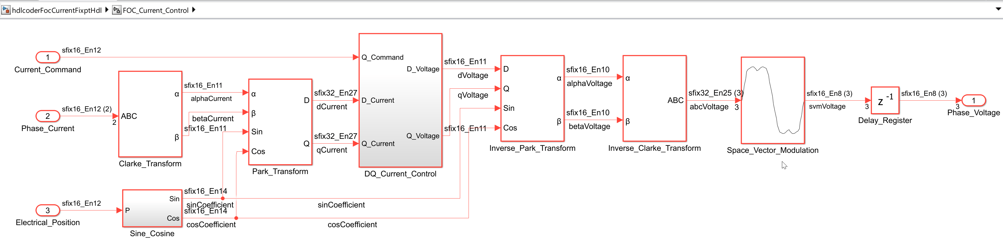
dut = "hdlcoderFocCurrentFixptHdl/FOC_Current_Control";

Configure and Establish the UltraScale+ Baseline

Establish a baseline on the AMD Zynq UltraScale+ device at a 100 MHz target. You compare the retargeted results against this baseline.

Configure the DUT and model for the baseline run:

• Enable improved adaptive pipelining and turn off distributed pipelining on the DUT.

• Add one input pipeline stage on the DUT.

• Set the model to treat rates as hardware rates so improved adaptive pipelining places its registers at the faster clock-rate domain.

• Set SubsystemReuse to off so the two PI current controllers inside DQ_Current_Control synthesize as independent hardware and each instance participates in pipelining decisions on its own.

• Enable CriticalPathEstimation so improved adaptive pipelining reports the paths that limit the achievable frequency.

matlab.internal.feature("GlobalAdaptivePipelining", 1);
hdlset_param(dut, "AdaptivePipelining",    "on");
hdlset_param(dut, "DistributedPipelining", "off");
hdlset_param(dut, "InputPipeline",         1);
hdlset_param(dut, "OutputPipeline",        0);

hdlset_param(model, ...
    "TargetLanguage",            "Verilog", ...
    "TargetFrequency",           100, ...
    "SynthesisTool",             "Xilinx Vivado", ...
    "SynthesisToolChipFamily",   "Zynq UltraScale+", ...
    "SynthesisToolDeviceName",   "xczu9eg", ...
    "SynthesisToolPackageName",  "ffvb1156", ...
    "SynthesisToolSpeedValue",   "-1", ...
    "CriticalPathEstimation",    "on", ...
    "TreatRatesAsHardwareRates", "on", ...
    "SubsystemReuse",            "off");

Generate HDL code for the baseline DUT:

makehdl(dut);

Confirm the estimate by running synthesis. For more information on HDL code generation and FPGA synthesis from a Simulink model, see HDL Code Generation and FPGA Synthesis from Simulink Model. The AMD Zynq UltraScale+ baseline reaches an Fmax of 105.83 MHz, above the 100 MHz target, with a worst-negative slack of +0.551 ns.

Retarget to PolarFire SoC Devices

Retarget the same DUT to the Microchip PolarFire SoC MPFS250T-FCG1152-1 device at the same 100 MHz target. Change only the synthesis target, generate code, examine the Critical Path Estimation (CPE) report, and then confirm the result with synthesis.

Change the synthesis tool and device parameters to retarget the same DUT to PolarFire SoC:

hdlset_param(model, ...
    "SynthesisTool",            "Microchip Libero SoC", ...
    "SynthesisToolChipFamily",  "PolarFireSoC", ...
    "SynthesisToolDeviceName",  "MPFS250T", ...
    "SynthesisToolPackageName", "FCG1152", ...
    "SynthesisToolSpeedValue",  "-1");

Generate HDL code for the retargeted DUT:

makehdl(dut);

The CPE report displays the path that critical path estimation identifies as limiting the achievable frequency and lists the blocks along it in propagation order. Use the report to decide where to add block-level pipelining. On this run, the report identifies a chain that begins at the Saturation_Magnitude block in Q_Current_Control, passes through a multiply-accumulate in Inverse_Park_Transform, and continues into a Gain in Inverse_Clarke_Transform. The estimated critical path shows a small positive slack that narrows during synthesis and place-and-route because the path is dominated by consecutive high-bit-width multiplies.

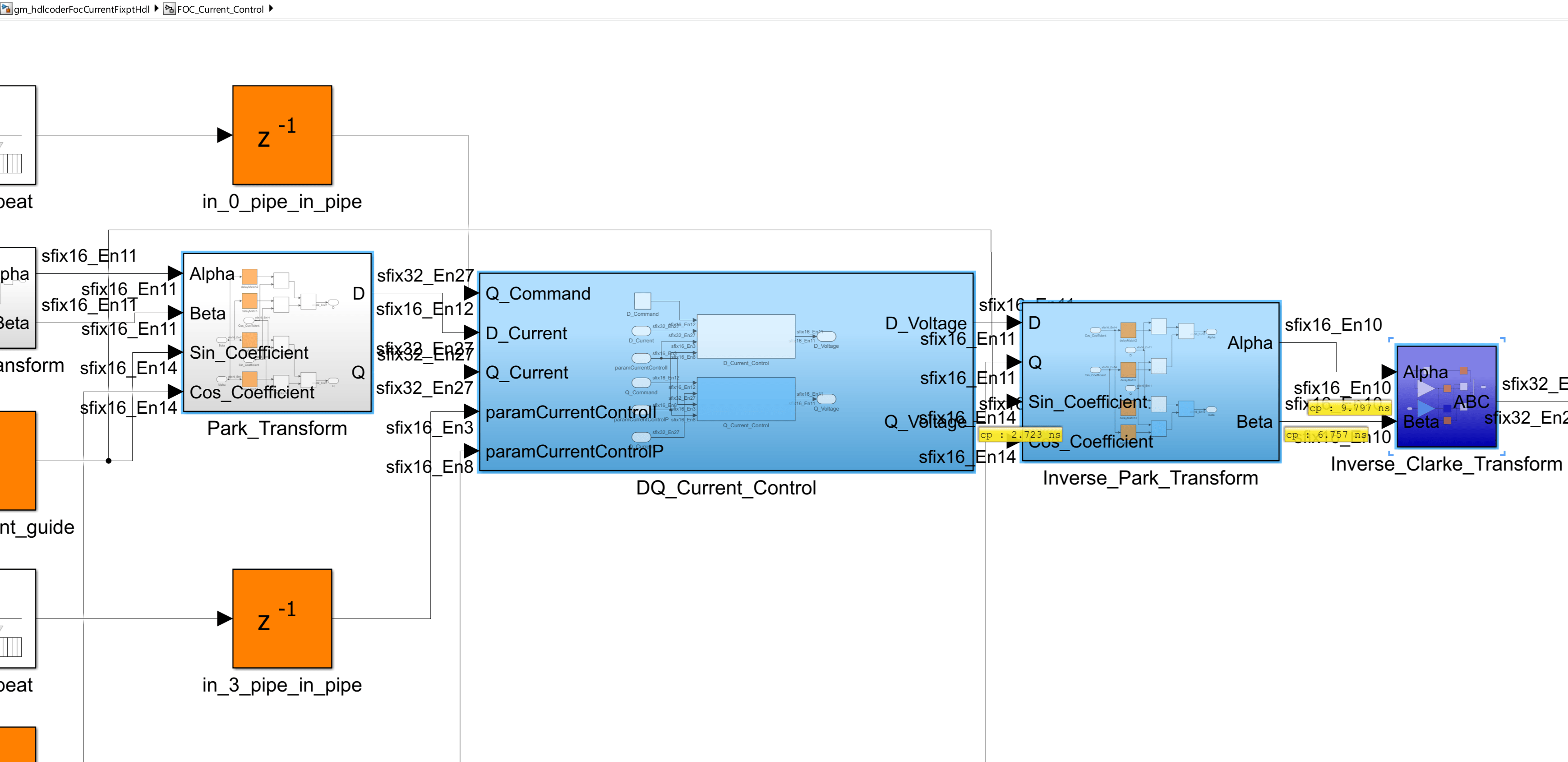
The CPE report lists the blocks along the critical path in propagation order. The cumulative propagation ends at the guide register at 9.797 ns, which results in +0.203 ns of estimated slack against the 10.000 ns budget.

Stage	Block	Delay (ns)	Cumulative Propagation (ns)
1	Saturation_Magnitude	0.000	0.000
2	Negate	0.941	0.941
3	Sat_LowerRelOp	0.769	1.710
4	Sat_LowerSwitch	0.525	2.235
5-9	Sat_UpperSwitch / Data_Type_Convert / Saturate_Output / Q_Current_Control / DQ_Current_Control	0.488	2.723
10	Product4 (Inverse_Park_Transform to Inverse_Clarke_Transform multiply-accumulate)	2.922	5.645
11	Add2	1.112	6.757
12-13	Gain1 (Inverse_Clarke_Transform multiply-accumulate)	2.922	9.679
14	Gain1_out1_guide (guide register)	0.118	9.797

This figure shows the FOC_Current_Control subsystem of the retargeted model, with the critical path highlighted.

Confirm the estimate by running synthesis. For more information on HDL code generation and FPGA synthesis from a Simulink model, see HDL Code Generation and FPGA Synthesis from Simulink Model. The initial retargeted run reaches an Fmax of 96.81 MHz, short of the 100 MHz target, with a worst-negative slack of -0.330 ns.

Adjust Block-Level Pipelining

The CPE-identified critical path passes through a multiply-accumulate in the Inverse_Park_Transform subsystem and continues into a Gain in the Inverse_Clarke_Transform subsystem. To break this multiply-accumulate chain, add an output pipeline stage to Inverse_Park_Transform, which lies on the path, and to Park_Transform, which feeds the current-control path upstream. Both subsystems contain a multiply-accumulate, which makes them good candidates for an output pipeline. Set OutputPipeline to 1 on both subsystems:

hdlset_param("hdlcoderFocCurrentFixptHdl/FOC_Current_Control/Park_Transform",         "OutputPipeline", 1);
hdlset_param("hdlcoderFocCurrentFixptHdl/FOC_Current_Control/Inverse_Park_Transform", "OutputPipeline", 1);

Regenerate HDL code with the adjustment applied:

makehdl(dut);

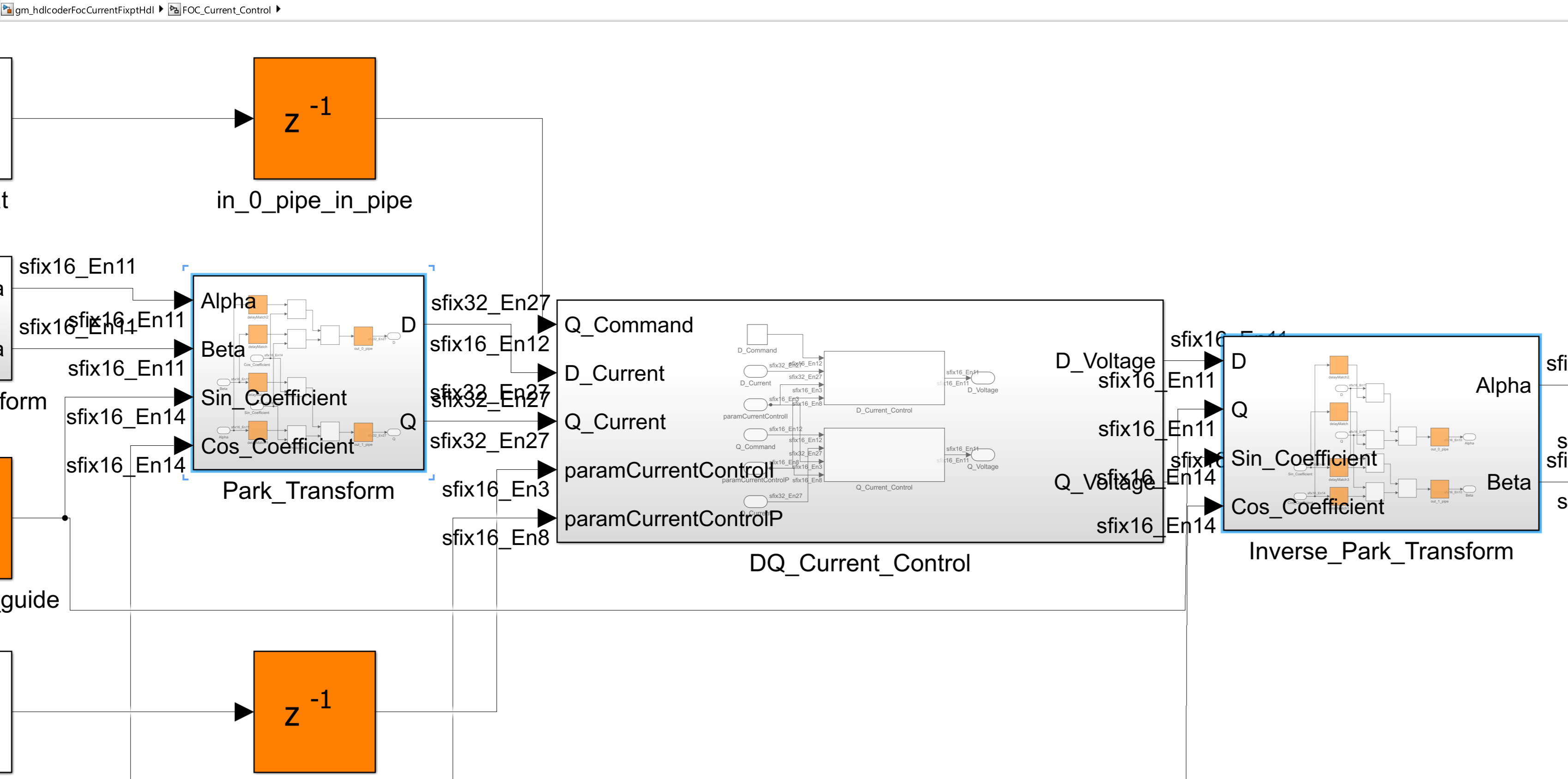
This figure shows the generated model after the two-line block-level pipelining adjustment. The Park_Transform and Inverse_Park_Transform subsystems show the additional output pipelines.

Regenerate the CPE report to see the effect of the adjustment. The estimated critical path relocates off the multiply-accumulate chain and onto the Sine_Cosine lookup path. The cumulative propagation now ends at the Sine_Cosine subsystem output at 9.307 ns, which results in +0.693 ns of estimated slack against the 10.000 ns budget. This table lists the blocks along the relocated path in propagation order:

Stage	Block	Delay (ns)	Cumulative Propagation (ns)
1	in_2_pipe_in_pipe (DUT input pipeline register)	0.336	0.336
2	Normalize_Position (Sine_Cosine)	2.922	3.258
3	CastU16En161 (Sine_Cosine_LUT)	0.000	3.258
4	Amp50 (Sine_Cosine_LUT)	0.941	4.199
5	QuadHandle1 (Sine_Cosine_LUT)	0.488	4.687
6	p50mA (Sine_Cosine_LUT)	1.016	5.703
7	QuadHandle21 (Sine_Cosine_LUT)	0.488	6.191
8	Look-Up Table1 (Sine_Cosine_LUT)	3.116	9.307
9-10	Sine_Cosine_LUT / Sine_Cosine (subsystem output)	0.000	9.307

Confirm the estimate by running synthesis. With this adjustment, improved adaptive pipelining reaches an Fmax of 118.57 MHz and closes 100 MHz timing with +1.566 ns of worst-negative slack. The DUT output latency remains 0 cycles because clock-rate pipelining absorbs the added registers into the oversampling headroom that the model creates from its faster clock-rate domain.

Compare Results Across Targets

Compare the synthesis results across the three runs. This table lists the synthesis data:

Target Device	Block-Level Pipelining Changes	Fmax (MHz)	WNS	Latency (Cycles)	DSP	LUT	FF
AMD Zynq UltraScale+ xczu9eg	InputPipeline=1 on DUT only	105.83	+0.551 ns	0	21	1218	637
Microchip PolarFire SoC MPFS250T	InputPipeline=1 on DUT only	96.81	-0.330 ns	0	21	2389	1721
Microchip PolarFire SoC MPFS250T with block-level pipelining	InputPipeline=1 on DUT, plus OutputPipeline=1 on Park_Transform and Inverse_Park_Transform	118.57	+1.566 ns	0	22	2294	1760

The AMD Zynq UltraScale+ device uses six-input LUTs and the Microchip PolarFire SoC device uses four-input LUTs, so the LUT counts are not directly comparable across the two targets. The DSP column reports the AMD DSP48E2 slices on the UltraScale+ device and Math blocks on the PolarFire SoC device.

Improved adaptive pipelining generalizes across both vendors on the same design and the same 100 MHz target. Because the PolarFire SoC device has a tighter timing requirements, critical path estimation helps identify the specific block-level path to address, and a two-line adjustment closes timing with margin.