このページは機械翻訳を使用して翻訳されました。最新版の英語を参照するには、ここをクリックします。

母集団多様性

母集団多様性の重要性

遺伝的アルゴリズムのパフォーマンスを決定する最も重要な要素の 1 つは、母集団の 多様性 です。個体間の平均距離が大きい場合、多様性は高くなります。平均距離が小さい場合、多様性は低くなります。適切な量の多様性を得るには、試行錯誤が必要です。多様性が高すぎたり低すぎたりすると、遺伝的アルゴリズムのパフォーマンスが悪くなる可能性があります。

このセクションでは、母集団の初期範囲を設定することで多様性を制御する方法について説明します。突然変異と交叉を変化させる のトピック「突然変異の量の設定」では、突然変異の量が多様性にどのように影響するかについて説明しています。

このセクションでは、母集団規模を設定する方法についても説明します。

初期範囲の設定

デフォルトでは、ga は作成関数を使用してランダムな初期母集団を作成します。InitialPopulationRange オプションで初期母集団内のベクトルの範囲を指定できます。

メモ: 初期範囲は、下限と上限を指定して、初期母集団内のポイントの範囲を制限します。後続の世代には、初期範囲に含まれないエントリを持つポイントが含まれる場合があります。lb および ub 入力引数を使用して、すべての世代の上限と下限を設定します。

問題の解決方法がおおよそわかっている場合は、解決方法の推測が含まれるように初期範囲を指定します。しかし、母集団に十分な多様性があれば、遺伝的アルゴリズムは、解が初期範囲内になくても解を見つけることができます。

この例では、初期範囲が遺伝的アルゴリズムのパフォーマンスにどのように影響するかを示します。この例では、ラストリギンの機能を最小限に抑える で説明されている Rastrigin 関数を使用します。関数の最小値は 0 であり、これは原点にあります。

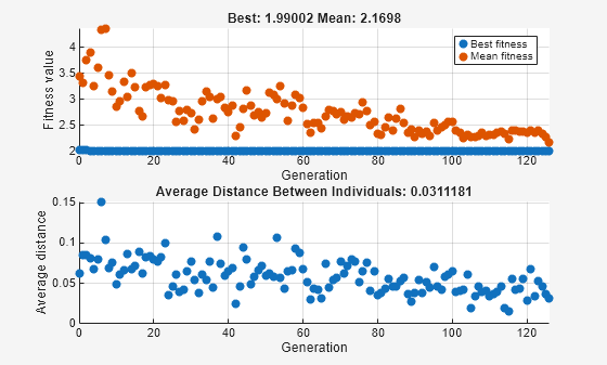
rng(1) % For reproducibility
fun = @rastriginsfcn;
nvar = 2;
options = optimoptions('ga','PlotFcn',{'gaplotbestf','gaplotdistance'},...
    'InitialPopulationRange',[1;1.1]);
[x,fval] = ga(fun,nvar,[],[],[],[],[],[],[],options)

ga stopped because the average change in the fitness value is less than options.FunctionTolerance.

x = 1×2

    0.9942    0.9950

fval = 
1.9900

上のグラフは各世代における最高の適応度を示しており、適応度値の低下がほとんど見られないことを示しています。下のグラフは各世代の個体間の平均距離を示しており、これは母集団の多様性を測る良い指標となります。この初期範囲の設定では、多様性が少なすぎるため、アルゴリズムが進行できません。

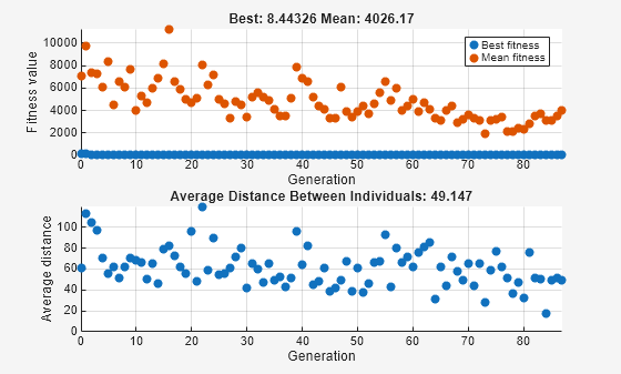
次に、InitialPopulationRangeを[1;100]に設定してみます。今回は結果がより多様です。現在の乱数設定では、かなり典型的な結果が生じます。

options.InitialPopulationRange = [1;100];
[x,fval] = ga(fun,nvar,[],[],[],[],[],[],[],options)

ga stopped because the average change in the fitness value is less than options.FunctionTolerance.

x = 1×2

   -2.1352   -0.0497

fval = 
8.4433

今回、遺伝的アルゴリズムは進歩しましたが、個体間の平均距離が非常に大きいため、最良の個体は最適解から遠く離れています。

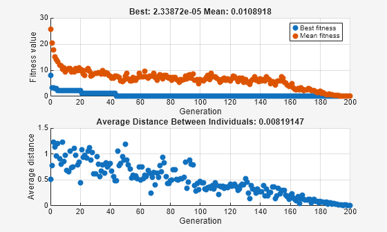
ここでInitialPopulationRangeを[1;2]に設定します。この設定は問題に適しています。

options.InitialPopulationRange = [1;2];
[x,fval] = ga(fun,nvar,[],[],[],[],[],[],[],options)

ga stopped because it exceeded options.MaxGenerations.

x = 1×2
10-3 ×

    0.2473   -0.2382

fval = 
2.3387e-05

適切な多様性により、通常、ga は前の 2 つのケースよりも良い結果を返します。

ga のカスタム プロット関数と線形制約

この例では、線形制約問題のデフォルトの作成関数である @gacreationlinearfeasible が ga の母集団を作成する方法を示します。母集団は広く分散しており、制約境界上に位置するように偏っています。この例では、カスタム プロット関数を使用します。

適応度関数

適応度関数は lincontest6 であり、この例を実行すると使用できます。lincontest6 は 2 つの変数の 2 次関数です。

カスタムプロット関数

次のコードを、MATLAB ® パスの gaplotshowpopulation2 という名前のファイルに保存します。

function state = gaplotshowpopulation2(~,state,flag,fcn)
%gaplotshowpopulation2 Plots the population and linear constraints in 2-d.
%   STATE = gaplotshowpopulation2(OPTIONS,STATE,FLAG) plots the population
%   in two dimensions.
%
%   Example:
%     fun = @lincontest6;
%     options = gaoptimset('PlotFcn',{{@gaplotshowpopulation2,fun}});
%     [x,fval,exitflag] = ga(fun,2,A,b,[],[],lb,[],[],options);

% This plot function works in 2-d only
if size(state.Population,2) > 2
    return;
end
if nargin < 4
    fcn = [];
end
% Dimensions to plot
dimensionsToPlot = [1 2];

switch flag
    % Plot initialization
    case 'init'
        pop = state.Population(:,dimensionsToPlot);
        plotHandle = plot(pop(:,1),pop(:,2),'*');
        set(plotHandle,'Tag','gaplotshowpopulation2')
        title('Population plot in two dimension','interp','none')
        xlabelStr = sprintf('%s %s','Variable ', num2str(dimensionsToPlot(1)));
        ylabelStr = sprintf('%s %s','Variable ', num2str(dimensionsToPlot(2)));
        xlabel(xlabelStr,'interp','none');
        ylabel(ylabelStr,'interp','none');
        hold on;
       
        % plot the inequalities
        plot([0 1.5],[2 0.5],'m-.') %  x1 + x2 <= 2
        plot([0 1.5],[1 3.5/2],'m-.'); % -x1 + 2*x2 <= 2
        plot([0 1.5],[3 0],'m-.'); % 2*x1 + x2 <= 3
        % plot lower bounds
        plot([0 0], [0 2],'m-.'); % lb = [ 0 0];
        plot([0 1.5], [0 0],'m-.'); % lb = [ 0 0];
        set(gca,'xlim',[-0.7,2.2])
        set(gca,'ylim',[-0.7,2.7])
        axx = gcf;
        % Contour plot the objective function
        if ~isempty(fcn)
            range = [-0.5,2;-0.5,2];
            pts = 100;
            span = diff(range')/(pts - 1);
            x = range(1,1): span(1) : range(1,2);
            y = range(2,1): span(2) : range(2,2);

            pop = zeros(pts * pts,2);
            values = zeros(pts,1);
            k = 1;
            for i = 1:pts
                for j = 1:pts
                    pop(k,:) = [x(i),y(j)];
                    values(k) = fcn(pop(k,:));
                    k = k + 1;
                end
            end
            values = reshape(values,pts,pts);
            contour(x,y,values);
            colorbar
        end
        % Show the initial population
        ax = gca;
        fig = figure;
        copyobj(ax,fig);colorbar
        % Pause for three seconds to view the initial plot, then resume
        figure(axx)
        pause(3);
    case 'iter'
        pop = state.Population(:,dimensionsToPlot);
        plotHandle = findobj(get(gca,'Children'),'Tag','gaplotshowpopulation2');
        set(plotHandle,'Xdata',pop(:,1),'Ydata',pop(:,2));
end

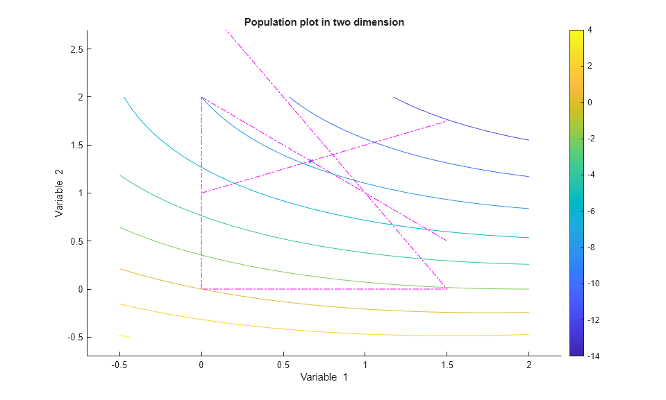
カスタム プロット関数は、線形不等式と境界制約を表す線をプロットし、適応度関数のレベル曲線をプロットし、母集団の進化をプロットします。このプロット関数は、通常の入力 (options,state,flag) だけでなく、この例では適応度関数への関数ハンドル @lincontest6 も必要とします。レベル曲線を生成するには、カスタム プロット関数に適応度関数が必要です。

問題の制約

境界と線形制約を含めます。

A = [1,1;-1,2;2,1];
b = [2;2;3];
lb = zeros(2,1);

プロット関数を含めるオプション

ga の実行時にプロット関数を含めるようにオプションを設定します。

options = optimoptions('ga','PlotFcns',...
{{@gaplotshowpopulation2,@lincontest6}});

問題を実行して母集団を観察する

最初のプロットにおける初期母集団には、線形制約境界上に多くのメンバーが存在します。母集団は適度に分散している。

rng default % for reproducibility
[x,fval] = ga(@lincontest6,2,A,b,[],[],lb,[],[],options);

ga stopped because the average change in the fitness value is less than options.FunctionTolerance.

ga は、解である単一の点に急速に収束します。

母集団規模の設定

Population オプションの Population size フィールドは、各世代における母集団のサイズを決定します。母集団数を増やすと、遺伝的アルゴリズムはより多くのポイントを探索できるようになり、より良い結果が得られます。ただし、母集団のサイズが大きくなるほど、遺伝的アルゴリズムが各世代を計算するのにかかる時間は長くなります。

メモ

各母集団内の個体が探索対象の空間にまたがるように、Population size を少なくとも 変数の数 の値に設定する必要があります。

実行に長時間を費やすことなく、良好な結果を返す Population size のさまざまな設定を試すことができます。

参考

トピック

• オプションと出力
• ga を使用したグローバル最適化とローカル最適化