このページは機械翻訳を使用して翻訳されました。最新版の英語を参照するには、ここをクリックします。

多目的最適化のためのパレート フロント、問題ベース

この例では、最適化変数を使用して多目的最適化問題を解決する方法と、解をプロットする方法を示します。

問題の定式化

この問題には、2 次元の最適化変数と 2 つの目的関数があります。最適化変数 x を、多目的ソルバーが期待する方向の行ベクトルとして作成します。x のコンポーネントの範囲が -50 から 50 になるように境界を設定します。

x = optimvar("x",1,2,LowerBound=-50,UpperBound=50);

2 つのコンポーネントの目的関数を作成します。最適化問題に目的関数を含めます。

fun(1) = x(1)^4 + x(2)^4 + x(1)*x(2) - x(1)^2*x(2)^2 - 9*x(1)^2;
fun(2) = x(1)^4 + x(2)^4 + x(1)*x(2) - x(1)^2*x(2)^2 + 3*x(2)^3;
prob = optimproblem("Objective",fun);

問題を確認します。

show(prob)

  OptimizationProblem : 

	Solve for:
       x

	minimize :
       ((((x(1).^4 + x(2).^4) + (x(1) .* x(2))) - (x(1).^2 .* x(2).^2)) - (9 .* x(1).^2))
       ((((x(1).^4 + x(2).^4) + (x(1) .* x(2))) - (x(1).^2 .* x(2).^2)) + (3 .* x(2).^3))


	variable bounds:
       -50 <= x(1) <= 50
       -50 <= x(2) <= 50

解を解き、プロットする

solve を呼び出してこの問題を解きます。

rng default % For reproducibility
sol = solve(prob)

Solving problem using gamultiobj.
gamultiobj stopped because the average change in the spread of Pareto solutions is less than options.FunctionTolerance.

sol = 
  1×18 OptimizationValues vector with properties:

   Variables properties:
            x: [2×18 double]

   Objective properties:
    Objective: [2×18 double]

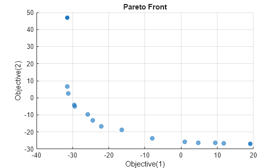
結果として得られるパレート フロントをプロットします。

paretoplot(sol)

paretosearch ソルバーを使用して問題を再度解きます。

sol2 = solve(prob,Solver="paretosearch");

Solving problem using paretosearch.

Pareto set found that satisfies the constraints. 

Optimization completed because the relative change in the volume of the Pareto set 
is less than 'options.ParetoSetChangeTolerance' and constraints are satisfied to within 
'options.ConstraintTolerance'.

paretoplot(sol2)

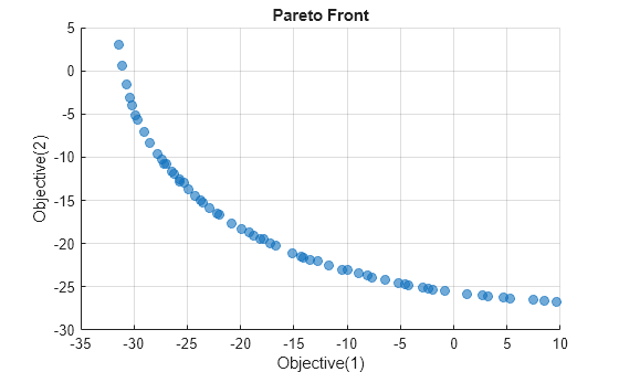
デフォルトのオプションを使用すると、paretosearch ソルバーは gamultiobj よりも密度の高いソリューション ポイントのセットを取得します。ただし、gamultiobj はより広い範囲の値を取得します。

単一目的のソリューションから始める

より広範囲のソリューションを実現するために、x = [1 1] から始まる単一目的ソリューションを見つけます。

x0.x = [1 1];
prob1 = optimproblem("Objective",fun(1));
solp1 = solve(prob1,x0);

Solving problem using fmincon.

Local minimum possible. Constraints satisfied.

fmincon stopped because the size of the current step is less than
the value of the step size tolerance and constraints are 
satisfied to within the value of the constraint tolerance.

<stopping criteria details>

prob2 = optimproblem("Objective",fun(2));
solp2 = solve(prob2,x0);

Solving problem using fmincon.

Local minimum found that satisfies the constraints.

Optimization completed because the objective function is non-decreasing in 
feasible directions, to within the value of the optimality tolerance,
and constraints are satisfied to within the value of the constraint tolerance.

<stopping criteria details>

solve の初期点として、単一目的のソリューションを準備します。各ポイントは列ベクトルとして optimvalues 関数に渡す必要があります。

start = optimvalues(prob,"x",[solp1.x' solp2.x']);

start ポイントから始めて、paretosearch を使用して多目的問題を解きます。

sol3 = solve(prob,start,Solver="paretosearch");

Solving problem using paretosearch.

Pareto set found that satisfies the constraints. 

Optimization completed because the relative change in the volume of the Pareto set 
is less than 'options.ParetoSetChangeTolerance' and constraints are satisfied to within 
'options.ConstraintTolerance'.

paretoplot(sol3)

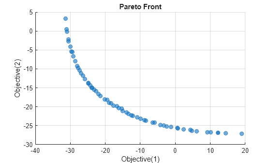
今回、paretosearch は目的関数のより広い範囲を見つけ、目的 2 ではほぼ 10 に、目的 1 ではほぼ 20 にまで達します。この範囲は、目標 1 = –31、目標 2 = 48 付近の異常な解点を除いて、gamultiobj範囲に似ています。

参考

gamultiobj | paretosearch | solve | paretoplot

トピック

• 多目的最適化