LMS アルゴリズムの使用による FIR フィルターのシステム同定

システム同定は、適応フィルターを使用して未知のシステムの係数を特定するプロセスです。このプロセスの概要は、システム同定 –– 適応フィルターの使用による未知のシステムの同定に示されています。関係する主なコンポーネントは以下のとおりです。

適応フィルターアルゴリズム。この例では、dsp.LMSFilter の Method プロパティを 'LMS' に設定して、LMS 適応フィルターアルゴリズムを選択します。
適応対象となる未知のシステムまたはプロセス。この例では、fircband で設計されたフィルターが未知のシステムです。
適応プロセスを実行する適切な入力データ。一般的な LMS モデルの場合、これらは目的の信号 $d (k)$ と入力信号 $x (k)$ です。

適応フィルターの目的は、適応フィルターの出力 $y (k)$ と未知のシステム (同定対象のシステム) の出力 $d (k)$ の間で誤差信号を最小化することです。誤差信号が最小化されると、適応させたフィルターは未知のシステムに似たものになります。両方のフィルターの係数は、ほぼ一致します。

メモ: R2016a 以前のリリースを使用している場合、それぞれのオブジェクトの呼び出しを等価な step 構文で置き換えてください。たとえば、obj(x) は step(obj,x) になります。

未知のシステム

同定対象のシステムを表す dsp.FIRFilter オブジェクトを作成します。関数 fircband を使用して、フィルターの係数を設計します。設計するフィルターは、阻止帯域で 0.2 リップルに制約されているローパスフィルターです。

filt = dsp.FIRFilter;
filt.Numerator = fircband(12,[0 0.4 0.5 1],[1 1 0 0],[1 0.2],... 
{'w' 'c'});

信号 x を FIR フィルターに渡します。目的の信号 d は、未知のシステム (FIR フィルター) の出力と加法性ノイズ信号 n の和です。

x = 0.1*randn(250,1);
n = 0.01*randn(250,1);
d = filt(x) + n;

適応フィルター

未知のフィルターを設計して目的の信号の準備ができたので、適応 LMS フィルターオブジェクトを作成および適用して未知のフィルターを特定します。

適応フィルターオブジェクトを準備するには、フィルターの係数を推定するための開始値と LMS のステップサイズ (mu) が必要です。フィルター係数の推定値として、一連の非ゼロ値で始めることができます。この例では、13 個のフィルターの重みの初期値にゼロを使用します。dsp.LMSFilter の InitialConditions プロパティをフィルターの重みの目的の初期値に設定します。ステップサイズについては、250 回の反復 (250 個の入力サンプル点) で適切に収束するための十分に大きい値と未知のフィルターを正確に推定するための十分に小さい値の間にある、0.8 が良い妥協点です。

LMS 適応アルゴリズムを使用する適応フィルターを表す dsp.LMSFilter オブジェクトを作成します。適応フィルターの長さを 13 タップ、ステップサイズを 0.8 に設定します。

mu = 0.8;
lms = dsp.LMSFilter(13,'StepSize',mu)

lms = 
  dsp.LMSFilter with properties:

                   Method: 'LMS'
                   Length: 13
           StepSizeSource: 'Property'
                 StepSize: 0.8000
            LeakageFactor: 1
        InitialConditions: 0
           AdaptInputPort: false
    WeightsResetInputPort: false
            WeightsOutput: 'Last'

  Show all properties

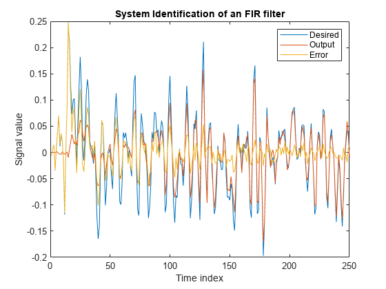
一次入力信号 x と目的の信号 d を LMS フィルターに渡します。適応フィルターを稼働させて、未知のシステムを特定します。適応フィルターの出力 y は目的の信号 d に収束された信号であり、2 つの信号間の誤差 e を最小化します。

結果をプロットします。出力信号と目的の信号が期待どおりには一致しておらず、これらの間の誤差は無視できません。

[y,e,w] = lms(x,d);
plot(1:250, [d,y,e])
title('System Identification of an FIR filter')
legend('Desired','Output','Error')
xlabel('Time index')
ylabel('Signal value')

Figure contains an axes object. The axes object with title System Identification of an FIR filter contains 3 objects of type line. These objects represent Desired, Output, Error.

重みの比較

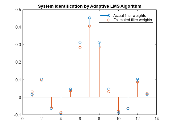
重みベクトル w は、未知のシステム (FIR フィルター) に似るように適応させた LMS フィルターの係数を表します。収束を確認するために、FIR フィルターの分子係数と適応フィルターの推定された重み付けを比較します。

前の信号プロットの結果を確認すると、推定されたフィルターの重みと実際のフィルターの重みが十分には一致していません。

stem([(filt.Numerator).' w])
title('System Identification by Adaptive LMS Algorithm')
legend('Actual filter weights','Estimated filter weights',...
       'Location','NorthEast')

Figure contains an axes object. The axes object with title System Identification by Adaptive LMS Algorithm contains 2 objects of type stem. These objects represent Actual filter weights, Estimated filter weights.

ステップサイズの変更

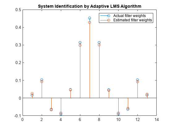
実験的に、ステップサイズを 0.2 に変更してみます。mu = 0.2 を使用して例を繰り返すと、以下のステムプロットが出力されます。フィルターは収束せず、推定された重みは実際の重みの良好な近似にはなっていません。

mu = 0.2;
lms = dsp.LMSFilter(13,'StepSize',mu);
[~,~,w] = lms(x,d);
stem([(filt.Numerator).' w])
title('System Identification by Adaptive LMS Algorithm')
legend('Actual filter weights','Estimated filter weights',...
       'Location','NorthEast')

データサンプル数の増加

目的の信号のフレームサイズを大きくします。これにより必要な計算量が増えますが、適応に使用できるデータがより多く LMS アルゴリズムに与えられます。信号データのサンプルを 1000 個、ステップサイズを 0.2 にすると、係数が前より一致するようになり、収束が改善されることがわかります。

release(filt);
x = 0.1*randn(1000,1);
n = 0.01*randn(1000,1);
d = filt(x) + n;
[y,e,w] = lms(x,d);
stem([(filt.Numerator).' w])
title('System Identification by Adaptive LMS Algorithm')
legend('Actual filter weights','Estimated filter weights',...
       'Location','NorthEast')

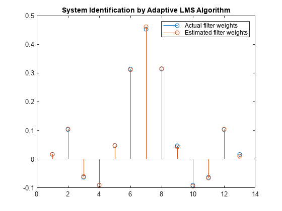
反復処理でデータを入力して、データサンプル数をさらに増やします。1000 サンプルずつまとめて 4 回の反復で渡して、4000 サンプルのデータに対して LMS アルゴリズムを実行します。

フィルターの重みを比較します。LMS フィルターの重みが FIR フィルターの重みと非常によく一致しているので、収束が適切であることがわかります。

release(filt);
n = 0.01*randn(1000,1);
for index = 1:4
  x = 0.1*randn(1000,1);
  d = filt(x) + n;
  [y,e,w] = lms(x,d);
end
stem([(filt.Numerator).' w])
title('System Identification by Adaptive LMS Algorithm')
legend('Actual filter weights','Estimated filter weights',...
       'Location','NorthEast')

出力信号と目的の信号が非常によく一致しており、これらの間の誤差はゼロに近くなっています。

plot(1:1000, [d,y,e])
title('System Identification of an FIR filter')
legend('Desired','Output','Error')
xlabel('Time index')
ylabel('Signal value')

Figure contains an axes object. The axes object with title System Identification of an FIR filter contains 3 objects of type line. These objects represent Desired, Output, Error.