最大および最小の活性化イメージを使用したイメージ分類の可視化

この例では、データセットを使用して何が深層ニューラルネットワークのチャネルを活性化するか発見する方法を説明します。これにより、ニューラルネットワークの仕組みを理解し、学習データセットの潜在的な問題を診断することができます。

この例では、食品のデータセットを転移学習させた GoogLeNet を使用して、いくつかのシンプルな可視化手法を取り上げます。分類器を最大あるいは最小に活性化させるイメージを確認することにより、ニューラルネットワークが誤った分類をする理由を見つけることができます。

データの読み込みと前処理

イメージをイメージデータストアとして読み込みます。この小さいデータセットには合計 978 の観測値と、食品の 9 つのクラスが含まれています。

このデータを学習セット、検証セット、およびテストセットに分割して、GoogLeNet を使用した転移学習の準備をします。

rng default
dataDir = fullfile(tempdir,"Food Dataset");
url = "https://www.mathworks.com/supportfiles/nnet/data/ExampleFoodImageDataset.zip";

if ~exist(dataDir,"dir")
    mkdir(dataDir);
end

downloadExampleFoodImagesData(url,dataDir);

Skipping download, file already exists...
Skipping unzipping, file already unzipped...
Done.

imds = imageDatastore(dataDir, ...
    "IncludeSubfolders",true,"LabelSource","foldernames");
[imdsTrain,imdsValidation,imdsTest] = splitEachLabel(imds,0.6,0.2);

学習データのクラス名を表示します。

classNames = categories(imdsTrain.Labels)

classNames = 9×1 cell
    {'caesar_salad' }
    {'caprese_salad'}
    {'french_fries' }
    {'greek_salad'  }
    {'hamburger'    }
    {'hot_dog'      }
    {'pizza'        }
    {'sashimi'      }
    {'sushi'        }

クラス数を表示します。

numClasses = numel(classNames)

numClasses = 9

データセットのイメージをいくつか選択して表示します。

rnd = randperm(numel(imds.Files),9);
for i = 1:numel(rnd)
subplot(3,3,i)
imshow(imread(imds.Files{rnd(i)}))
label = imds.Labels(rnd(i));
title(label,"Interpreter","none")
end

食品イメージを分類するネットワークの学習

事前学習済みの GoogLeNet ネットワークと対応するクラス名を読み込みます。これには、Deep Learning Toolbox™ Model for GoogLeNet Network サポートパッケージが必要です。このサポートパッケージがインストールされていない場合、ソフトウェアによってダウンロード用リンクが表示されます。使用可能なすべてのネットワークについては、事前学習済みの深層ニューラルネットワークを参照してください。

ネットワークの畳み込み層は、入力イメージを分類するために、最後の学習可能な層と最終ソフトマックス層が使用するイメージの特徴を抽出します。GoogLeNet のこれらの 2 つの層 'loss3-classifier' および 'prob' は、ネットワークによって抽出された特徴を組み合わせてクラス確率、損失値、および予測ラベルにまとめる方法に関する情報を含んでいます。新しいデータの再学習の準備ができているニューラルネットワークを返すには、クラスの数も指定します。

net = imagePretrainedNetwork("googlenet","NumClasses",numClasses);

新しい全結合層の学習率を増やします。

fcLayer = net.Layers(end-1);
fcLayer.WeightLearnRateFactor = 10;
fcLayer.BiasLearnRateFactor = 10;
net = replaceLayer(net,fcLayer.Name,fcLayer);

ネットワークの Layers プロパティの最初の要素はイメージ入力層です。この層にはサイズが 224 x 224 x 3 の入力イメージが必要です。ここで、3 はカラーチャネルの数です。

inputSize = net.Layers(1).InputSize;

ネットワークの学習

ネットワークにはサイズが 224 x 224 x 3 の入力イメージが必要ですが、イメージデータストアにあるイメージのサイズは異なります。拡張イメージデータストアを使用して学習イメージのサイズを自動的に変更します。学習イメージに対して実行する追加の拡張演算として、学習イメージを縦軸に沿ってランダムに反転させる演算、最大 30 ピクセルだけランダムに平行移動させる演算、および水平方向と垂直方向に最大 10% スケールアップする演算を指定します。データ拡張は、ネットワークで過適合が発生したり、学習イメージの正確な詳細が記憶されたりすることを防止するのに役立ちます。

pixelRange = [-30 30];
scaleRange = [0.9 1.1];
imageAugmenter = imageDataAugmenter( ...
    'RandXReflection',true, ...
    'RandXTranslation',pixelRange, ...
    'RandYTranslation',pixelRange, ...
    'RandXScale',scaleRange, ...
    'RandYScale',scaleRange);
augimdsTrain = augmentedImageDatastore(inputSize(1:2),imdsTrain, ...
    'DataAugmentation',imageAugmenter);

他のデータ拡張を実行せずに検証イメージのサイズを自動的に変更するには、追加の前処理演算を指定せずに拡張イメージデータストアを使用します。

augimdsValidation = augmentedImageDatastore(inputSize(1:2),imdsValidation);

学習オプションを指定します。オプションの中から選択するには、経験的解析が必要です。実験を実行してさまざまな学習オプションの構成を調べるには、Experiment Managerアプリを使用できます。

SGDM オプティマイザーを使用して学習させます。
InitialLearnRate を小さい値に設定して、まだ凍結されていない転移層での学習速度を下げます。上記の手順では、最後の学習可能な層の学習率係数を大きくして、新しい最後の層での学習時間を短縮しています。この学習率設定の組み合わせによって、新しい層では高速に学習が行われ、中間層では学習速度が低下し、凍結された初期の層では学習が行われません。
学習するエポック数を指定します。転移学習の実行時には、同じエポック数の学習を行う必要はありません。エポックとは、学習データセット全体の完全な学習サイクルのことです。
ミニバッチのサイズと検証データを指定します。エポックごとに 1 回、検定精度を計算します。
学習の進行状況をプロットで表示し、精度を監視します。
詳細出力を無効にします。

miniBatchSize = 10;
valFrequency = floor(numel(augimdsTrain.Files)/miniBatchSize);
options = trainingOptions('sgdm', ...
    'MiniBatchSize',miniBatchSize, ...
    'MaxEpochs',4, ...
    'InitialLearnRate',3e-4, ...
    'Shuffle','every-epoch', ...
    'ValidationData',augimdsValidation, ...
    'ValidationFrequency',valFrequency, ...
    'Plots','training-progress', ...
    'Metric',"accuracy",...
    'Verbose',false);

関数 trainnet を使用してニューラルネットワークに学習させます。分類には、クロスエントロピー損失を使用します。既定では、関数 trainnet は利用可能な GPU がある場合にそれを使用します。GPU での学習には、Parallel Computing Toolbox™ ライセンスとサポートされている GPU デバイスが必要です。サポートされているデバイスについては、GPU 計算の要件 (Parallel Computing Toolbox)を参照してください。そうでない場合、関数 trainnet は CPU を使用します。実行環境を指定するには、ExecutionEnvironment 学習オプションを使用します。このデータセットは小さいため、学習は短時間で終了します。実際にこの例を実行してネットワークに学習させた場合、学習過程に含まれるランダム性のため、異なる結果が得られ誤分類をする可能性があります。

net = trainnet(augimdsTrain,net,"crossentropy",options);

テストイメージの分類

テストイメージを分類し、分類精度を計算します。複数の観測値を使用して予測を行うには、関数 minibatchpredict を使用します。予測スコアをラベルに変換するには、関数 scores2label を使用します。関数 minibatchpredict は利用可能な GPU がある場合に自動的にそれを使用します。GPU を使用するには、Parallel Computing Toolbox™ ライセンスとサポートされている GPU デバイスが必要です。サポートされているデバイスについては、GPU 計算の要件 (Parallel Computing Toolbox)を参照してください。そうでない場合、関数は CPU を使用します。

augimdsTest = augmentedImageDatastore(inputSize(1:2),imdsTest);

predictedScores = minibatchpredict(net,augimdsTest);
predictedClasses = scores2label(predictedScores,classNames);

accuracy = mean(predictedClasses == imdsTest.Labels)

accuracy = 0.8980

テストセットの混同行列

テストセットの予測の混同行列をプロットします。これは、ネットワークで最も問題の原因になっているクラスを強調表示します。

figure;
confusionchart(imdsTest.Labels,predictedClasses,'Normalization',"row-normalized");

混同行列は、グリークサラダ、刺身、ホットドッグ、寿司といったいくつかのクラスに対するネットワーク性能が低いことを示しています。これらのクラスはデータセット内で少数しか存在しないため、そのことがネットワーク性能に影響を与えている可能性があります。ネットワーク性能が上がらない原因をより深く理解するため、これらのクラスのいずれかを調査します。

figure();
histogram(imdsValidation.Labels);
ax = gca();
ax.XAxis.TickLabelInterpreter = "none";

分類の調査

ネットワークによる寿司クラスの分類について調査します。

最も寿司らしい寿司

最初に、ネットワークの寿司クラスを最も強く活性化する寿司のイメージを探します。これは、"ネットワークはどのイメージを最も寿司らしいと考えるか" という質問の答えになります。

最大に活性化するイメージ、すなわち、全結合層の "寿司" ニューロンを強く活性化する入力イメージをプロットします。次の Figure は上位 4 つのイメージをクラススコアの降順に示しています。

chosenClass = "sushi";
classIdx = find(classNames == chosenClass);

numImgsToShow = 4;

[sortedScores,imgIdx] = findMaxActivatingImages(imdsTest,chosenClass,predictedScores,numImgsToShow);

figure
plotImages(imdsTest,imgIdx,sortedScores,predictedClasses,numImgsToShow)

寿司クラスの手がかりの可視化

ネットワークは寿司について正しい部分に着目しているでしょうか。ネットワークの寿司クラスで最大に活性化されたイメージは、相互に類似しており、多くの円形のものが互いに密集しています。

ネットワークはこのような種類の寿司を上手く分類しています。しかし、これが正しいことを検証し、ネットワークの判定理由をより正確に理解するには、Grad-CAM のような可視化手法を使用します。Grad-CAM の使用の詳細については、Grad-CAM での深層学習による判定の理由の解明を参照してください。

拡張イメージデータストアから最初のサイズ変更されたイメージを読み取り、gradCAM を使用して Grad-CAM による可視化をプロットします。

imageNumber = 1;

observation = augimdsTest.readByIndex(imgIdx(imageNumber));
img = observation.input{1};

label = predictedClasses(imgIdx(imageNumber));
score = sortedScores(imageNumber);

gradcamMap = gradCAM(net,img,label);

figure
alpha = 0.5;
plotGradCAM(img,gradcamMap,alpha);
sgtitle(string(label)+" (score: "+ max(score)+")")

Grad-CAM マップを見ると、ネットワークがイメージ内の寿司に焦点を当てていることがわかります。ただし、ネットワークが皿やテーブルの一部を見ていることもわかります。

最も寿司らしくない寿司

今度は、寿司クラスについてネットワークを最も活性化しない寿司のイメージを探します。これは、"ネットワークはどのイメージを最も寿司らしくないと考えるか" という質問の答えになります。それらのイメージのうちのいくつか (イメージ 3 や 4 など) には実際に刺身が含まれています。これは、実はネットワークが誤分類したわけではないことを意味します。これらのイメージには誤ったラベルが付いています。

ネットワークの性能が劣るイメージを見つけ、その判定に関する洞察が得られるため、これは有用です。

chosenClass = "sushi";
numImgsToShow = 9;

[sortedScores,imgIdx] = findMinActivatingImages(imdsTest,chosenClass,predictedScores,numImgsToShow);

figure
plotImages(imdsTest,imgIdx,sortedScores,predictedClasses,numImgsToShow)

刺身に誤分類された寿司の調査

なぜネットワークは寿司を誤って分類するのでしょうか。ネットワークが何に焦点を当てているかを確認するには、これらのイメージの 1 つに対して Grad-CAM 手法を実行します。

imageNumber = 4;
observation = augimdsTest.readByIndex(imgIdx(imageNumber));
img = observation.input{1};

label = predictedClasses(imgIdx(imageNumber));
score = sortedScores(imageNumber);

gradcamMap = gradCAM(net,img,label);

figure
alpha = 0.5;
plotGradCAM(img,gradcamMap,alpha);
title(string(label)+" (sushi score: "+ max(score)+")")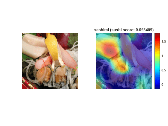

予想どおり、ネットワークは寿司ではなく刺身に焦点を当てています。

まとめ

クラススコアの大小を決めるデータ点や、ネットワークが高い信頼度で誤分類をするデータ点を調査することは、学習済みのネットワークがどのように機能しているかに関して有用な洞察が得られるシンプルな手法です。食品のデータセットの場合、この例では次のことが明確になりました。

テストデータには、実際は "寿司" であっても "刺身" というように、真のラベルが誤っているイメージが複数含まれる。このデータには、寿司と刺身の両方が含まれるイメージのように、不完全なラベルも含まれている。
ネットワークは "寿司" を "複数の集合した円形のもの" と考えている。しかし、単独の寿司も同様に区別できなければならない。
性能を改善するには、少数しか存在しないクラスのイメージをさらに数多くネットワークに見せる必要がある。

補助関数

function downloadExampleFoodImagesData(url,dataDir)
% Download the Example Food Image data set, containing 978 images of
% different types of food split into 9 classes.

% Copyright 2019 The MathWorks, Inc.

fileName = "ExampleFoodImageDataset.zip";
fileFullPath = fullfile(dataDir,fileName);

% Download the .zip file into a temporary directory.
if ~exist(fileFullPath,"file")
    fprintf("Downloading MathWorks Example Food Image dataset...\n");
    fprintf("This can take several minutes to download...\n");
    websave(fileFullPath,url);
    fprintf("Download finished...\n");
else
    fprintf("Skipping download, file already exists...\n");
end

% Unzip the file.
%
% Check if the file has already been unzipped by checking for the presence
% of one of the class directories.
exampleFolderFullPath = fullfile(dataDir,"pizza");
if ~exist(exampleFolderFullPath,"dir")
    fprintf("Unzipping file...\n");
    unzip(fileFullPath,dataDir);
    fprintf("Unzipping finished...\n");
else
    fprintf("Skipping unzipping, file already unzipped...\n");
end
fprintf("Done.\n");

end

function [sortedScores,imgIdx] = findMaxActivatingImages(imds,className,predictedScores,numImgsToShow)
% Find the predicted scores of the chosen class on all the images of the chosen class
% (e.g. predicted scores for sushi on all the images of sushi)
[scoresForChosenClass,imgsOfClassIdxs] = findScoresForChosenClass(imds,className,predictedScores);

% Sort the scores in descending order
[sortedScores,idx] = sort(scoresForChosenClass,'descend');

% Return the indices of only the first few
imgIdx = imgsOfClassIdxs(idx(1:numImgsToShow));

end

function [sortedScores,imgIdx] = findMinActivatingImages(imds,className,predictedScores,numImgsToShow)
% Find the predicted scores of the chosen class on all the images of the chosen class
% (e.g. predicted scores for sushi on all the images of sushi)
[scoresForChosenClass,imgsOfClassIdxs] = findScoresForChosenClass(imds,className,predictedScores);

% Sort the scores in ascending order
[sortedScores,idx] = sort(scoresForChosenClass,'ascend');

% Return the indices of only the first few
imgIdx = imgsOfClassIdxs(idx(1:numImgsToShow));

end

function [scoresForChosenClass,imgsOfClassIdxs] = findScoresForChosenClass(imds,className,predictedScores)
% Find the index of className (e.g. "sushi" is the 9th class)
uniqueClasses = unique(imds.Labels);
chosenClassIdx = string(uniqueClasses) == className;

% Find the indices in imageDatastore that are images of label "className"
% (e.g. find all images of class sushi)
imgsOfClassIdxs = find(imds.Labels == className);

% Find the predicted scores of the chosen class on all the images of the
% chosen class
% (e.g. predicted scores for sushi on all the images of sushi)
scoresForChosenClass = predictedScores(imgsOfClassIdxs,chosenClassIdx);
end

function plotImages(imds,imgIdx,sortedScores,predictedClasses,numImgsToShow)

for i=1:numImgsToShow
    score = sortedScores(i);
    sortedImgIdx = imgIdx(i);
    predClass = predictedClasses(sortedImgIdx); 
    correctClass = imds.Labels(sortedImgIdx);
        
    imgPath = imds.Files{sortedImgIdx};
    
    if predClass == correctClass
        color = "\color{green}";
    else
        color = "\color{red}";
    end
    
    predClassTitle = strrep(string(predClass),'_',' ');
    correctClassTitle = strrep(string(correctClass),'_',' ');
    
    subplot(3,ceil(numImgsToShow./3),i)
    imshow(imread(imgPath));
    title("Predicted: " + color + predClassTitle + "\newline\color{black}Score: " + num2str(score) + "\newlineGround truth: " + correctClassTitle);
end

end

function plotGradCAM(img,gradcamMap,alpha)

subplot(1,2,1)
imshow(img);

h = subplot(1,2,2);
imshow(img)
hold on;
imagesc(gradcamMap,'AlphaData',alpha);

originalSize2 = get(h,'Position');

colormap jet
colorbar

set(h,'Position',originalSize2);
hold off;
end

参考