Prune and Quantize Convolutional Neural Network for Speech Recognition
This example shows how to compress a convolutional neural network (CNN) to prepare it for deployment on an embedded system.
Deploying deep learning models on embedded systems can be challenging due to the limited memory and processing power of embedded systems. Model compression addresses these limitations by reducing the memory footprint of a model.
This example covers two model compression techniques for deep learning models: pruning and quantization. Pruning with a Taylor pruning algorithm removes convolution filters to reduce the size of the network and increase the inference speed. Quantizing the weights, biases, and activations of the layer to 8-bit scaled integer data types further reduces the memory requirement of the network.
The network you use in this example is trained to recognize speech commands. For more information, see Train Deep Learning Network for Speech Command Recognition (Audio Toolbox).
Load Data
This example uses the Google Speech Commands Dataset [1]. Download and unzip the data set.
downloadFolder = matlab.internal.examples.downloadSupportFile("audio","google_speech.zip");
dataFolder = tempdir;
unzip(downloadFolder,dataFolder)
dataset = fullfile(dataFolder,"google_speech");
Create Training and Validation Data
Create training and validation datastores before loading the pretrained network. This section follows the steps in Train Deep Learning Network for Speech Command Recognition (Audio Toolbox) to augment the data, create datastores, and extract auditory spectrograms.
The network must be able to not only recognize different spoken words but also to detect if the audio input is silence or background noise.
The supporting function augmentDataset uses the long audio files in the background folder of the Google Speech Commands Dataset to create one-second segments of background noise. The function creates an equal number of background segments from each background noise file and then splits the segments between the training and validation folders.
augmentDataset(dataset);
Progress = 17 (%)
Progress = 33 (%)
Progress = 50 (%)
Progress = 67 (%)
Progress = 83 (%)
Progress = 100 (%)
Use the supporting function createDatastores to create training and validation datastores. The function accepts a categorical array specifying the words that you want your model to recognize as commands and returns training and validation datastores, adsTrain and adsValidation.
commands = categorical(["yes","no","up","down","left","right","on","off","stop","go"]);
[adsTrain,adsValidation] = createDatastores(dataset,commands);
Use the supporting function extractFeatures to extract the auditory spectrograms from the audio input. XTrain contains the spectrograms from the training datastore and XValidation contains the spectrograms from the validation datastore. TTrain and TValidation are the training and validation target labels, isolated for convenience. Use categories to extract the class names.
[XTrain,XValidation,TTrain,TValidation] = extractFeatures(adsTrain,adsValidation);
classes = categories(TTrain);
Load Pretrained Network
Load the trained network.
load("trainedCommandNet.mat")Evaluate Trained Network
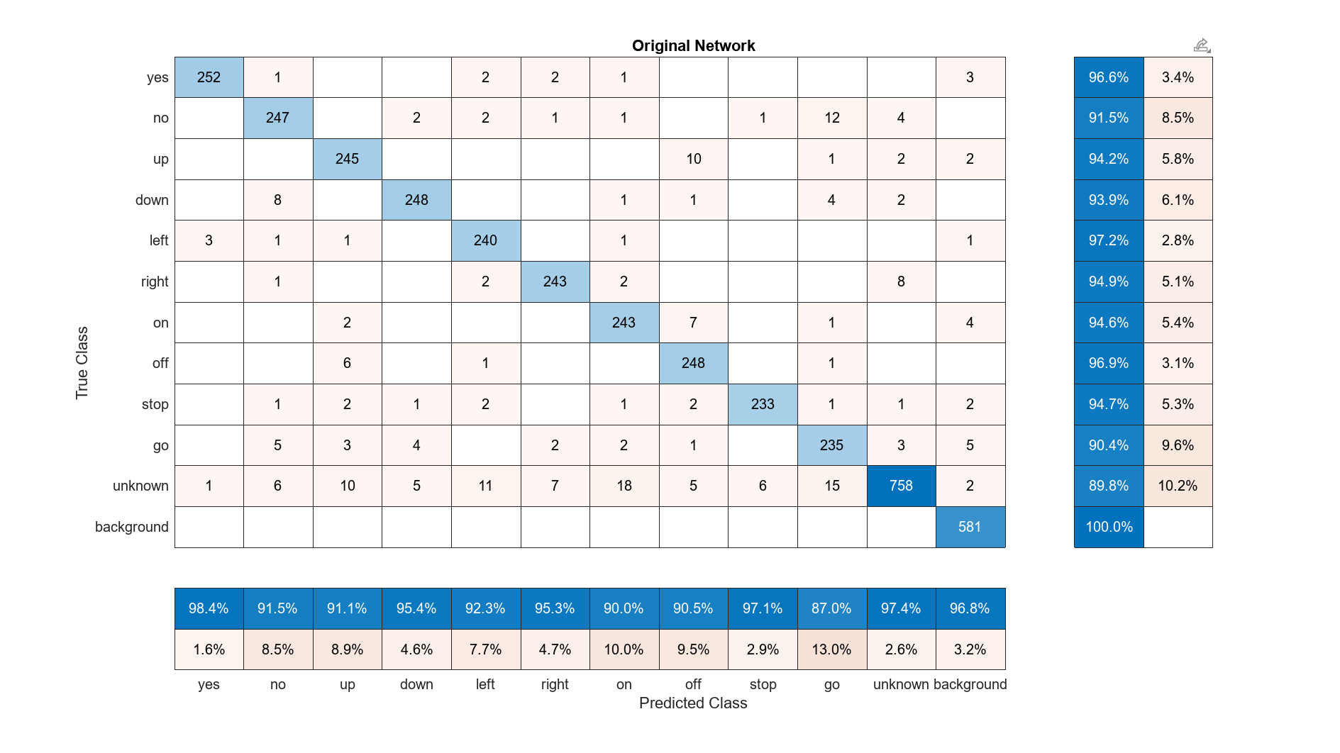
Use the networkAccuracy function to calculate the network accuracy and plot a confusion matrix for the validation set.
trainAccuracy = networkAccuracy(trainedNet,XTrain,TTrain,XValidation,TValidation,classes,commands,"Original Network"); "Training Accuracy: 96.0745%"
"Validation Accuracy: 93.5162%"

Prepare Network and Data for Pruning
Create datastores dsTrain and dsValidation from the spectrograms used for network training and validation.
classWeights = 1./countcats(TTrain);
classWeights = classWeights'/mean(classWeights);
dsTrain = augmentedImageDatastore([98 50], XTrain, TTrain);
dsValidation = augmentedImageDatastore([98 50], XValidation, TValidation);
Create minibatchqueue objects for the training and validation data for use in the custom pruning loops.
miniBatchSize = 50;

executionEnvironment = "auto";

mbqTrain = minibatchqueue(dsTrain, ...
    MiniBatchSize=miniBatchSize, ...
    MiniBatchFcn=@preprocessMiniBatch, ...
    MiniBatchFormat=["SSCB",""]);

mbqValidation = minibatchqueue(dsValidation, ...
    MiniBatchSize=miniBatchSize, ...
    MiniBatchFcn=@preprocessMiniBatch, ...
    MiniBatchFormat=["SSCB",""]);
Prune Network
Reduce the overall size of the network by pruning it using a Taylor pruning algorithm. For more information about Taylor pruning, see Prune Image Classification Network Using Taylor Scores.
Convert the network to a taylorPrunableNetwork object.
prunableNet = taylorPrunableNetwork(trainedNet);
Specify Pruning and Fine-Tuning Options
Set the pruning options.
maxPruningIterationssets the maximum number of iterations to be used for pruning process.maxToPrunesets the maximum number of filters to be pruned in each iteration of the pruning cycle.
maxPruningIterations = 16;
maxToPrune = 8;
maxPrunableFilters = prunableNet.NumPrunables;
numTest = size(TValidation,1);
minPrunables = 5;
Set the fine-tuning options.
learnRate = 1e-2;
momentum = 0.9;
numMinibatchUpdates = 50;
validationFrequency = 1;
Prune Network
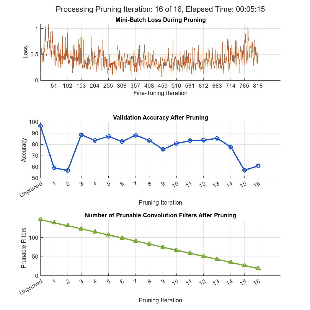
Prune the network. The taylorPruningLoop function defines the pruning iterations for each mini-batch. Each pruning iteration performs these steps:
Evaluate the pruning activations, gradients of the pruning activations, model gradients, state, and loss.
Update the network state.
Update the network parameters according to the optimizer.
Compute first-order Taylor scores and accumulate scores across previous batches of data.
Display progress.
prunableNet = taylorPruningLoop(prunableNet, mbqTrain, mbqValidation, classes, classWeights, numTest, maxPruningIterations, ...
                                maxPrunableFilters, maxToPrune, minPrunables, learnRate, ...
                                momentum, numMinibatchUpdates, validationFrequency,trainAccuracy);

The pruned network has a lower validation accuracy than the original network. To regain accuracy, you can retrain the network.
Retrain Pruned Network
Convert the pruned network to a dlnetwork.
prunedNet = dlnetwork(prunableNet)
prunedNet =
  dlnetwork with properties:

         Layers: [23×1 nnet.cnn.layer.Layer]
    Connections: [22×2 table]
     Learnables: [22×3 table]
          State: [10×3 table]
     InputNames: {'imageinput'}
    OutputNames: {'softmax'}
    Initialized: 1

  View summary with summary.
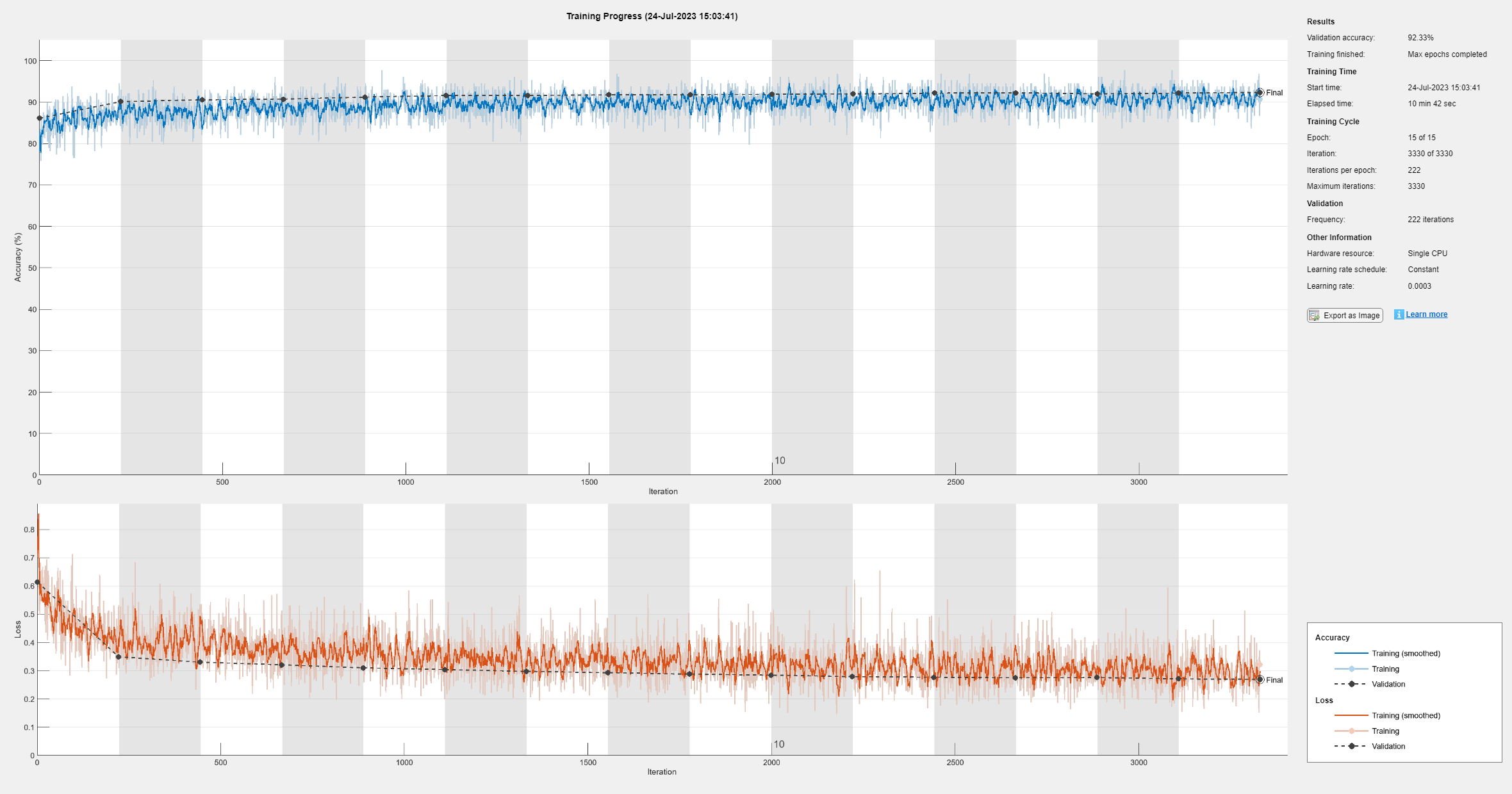
Specify training options.
miniBatchSize = 128;
validationFrequency = floor(numel(TTrain)/miniBatchSize);
options = trainingOptions("sgdm", ...
    InitialLearnRate=1e-3, ...
    MaxEpochs=30, ...
    LearnRateDropFactor=0.1, ...
    LearnRateDropPeriod=5, ...
    MiniBatchSize=miniBatchSize, ...
    Shuffle="every-epoch", ...
    Plots="training-progress", ...
    Verbose=false, ...
    ValidationData={XValidation,TValidation}, ...
    OutputNetwork="best-validation-loss", ...
    ValidationFrequency=validationFrequency, ...
    Metrics="accuracy");
To give each class equal total weight in the loss, use class weights that are inversely proportional to the number of training examples in each class. Train the network using trainnet.
lossfcn = @(Y,T)crossentropy(Y,T,classWeights(:),WeightsFormat="C");
trainedNetPruned = trainnet(XTrain,TTrain,prunedNet,lossfcn,options);
Evaluate Pruned Network
Calculate the accuracy of the pruned network after retraining and plot the confusion matrix. Compare the accuracy of the original network and the pruned network.
networkAccuracy(trainedNetPruned,XTrain,TTrain,XValidation,TValidation,classes,commands,"Pruned Network"); "Training Accuracy: 94.5106%"
"Validation Accuracy: 92.5686%"

The accuracy of the retrained pruned network is similar to the accuracy of the original network. You can interpret the slight decrease in accuracy as trimming the model, removing predictive capacity that does not specifically help distinguish your chosen keywords from other inputs. Comparing the confusion charts of the two networks shows that the retrained pruned network performs slightly better than the original network in some classes and worse in others. In other words, the pruned network has a reduced model size and complexity but is still able to perform the desired task.
Quantize Pruned Network
Create a dlquantizer object from the pruned network and specify the ExecutionEnvironment property as "GPU" to prepare for deployment to a GPU device.
dlquantObj = dlquantizer(trainedNetPruned,ExecutionEnvironment='GPU');Collect calibration statistics. Use the supporting function createCalibrationSet to create a representative calibration datastore with elements from each label in the training data.
calData = createCalibrationSet(XTrain,TTrain,36,["yes","no","up","down","left","right","on","off","stop","go","unknown","background"]);
calibrate(dlquantObj, calData);
Quantize the network with the quantize function.
qnetPruned = quantize(dlquantObj,ExponentScheme="Histogram");
save("qnet","qnetPruned")
qDetails = quantizationDetails(qnetPruned)
qDetails = struct with fields:
            IsQuantized: 1
          TargetLibrary: "cudnn"
    QuantizedLayerNames: [20×1 string]
    QuantizedLearnables: [10×3 table]
Evaluate Quantized Network
Calculate the accuracy of the quantized pruned network and plot the confusion matrix.
networkAccuracy(qnetPruned,XTrain,TTrain,XValidation,TValidation,classes,commands,"Pruned and Quantized Network"); "Training Accuracy: 94.486%"
"Validation Accuracy: 92.3691%"

Compare the accuracy of the pruned network before and after quantization. The training accuracy experiences a small decrease, and the validation accuracy remains constant.
Evaluate Network Compression
Use the estimateNetworkMetrics function to generate network metrics for the original network, the pruned network, and the quantized network.
originalNetMetrics = estimateNetworkMetrics(trainedNet);
taylorNetMetrics = estimateNetworkMetrics(trainedNetPruned);
quantizedNetMetrics = estimateNetworkMetrics(qnetPruned);
Evaluate the impact of each stage of compression on the number of learnables in the network.
Extract the number of learnable parameters in each network and visualize them in a bar plot.
figure
learnables = [sum(originalNetMetrics.NumberOfLearnables)
               sum(taylorNetMetrics.NumberOfLearnables)
               sum(quantizedNetMetrics.NumberOfLearnables)];

x = categorical({'Original','Taylor Pruned','Quantized'});
x = reordercats(x, string(x));
plotResults(x, learnables)
ylabel("Number of Learnables")
title("Number of Learnables in Network")
The plot shows that filter pruning is responsible for the reduction in the number of learnables. Quantization yields no reduction.
Evaluate the impact of each stage of compression on the parameter memory of the network.
Extract the parameter memory of each network and visualize the values in a bar plot.
figure;
memory = [sum(originalNetMetrics.("ParameterMemory (MB)"))
               sum(taylorNetMetrics.("ParameterMemory (MB)"))
               sum(quantizedNetMetrics.("ParameterMemory (MB)"))];

plotResults(x, memory)
ylabel("Parameter Memory (MB)")
title("Parameter Memory of Network")

Pruning greatly reduces the parameter memory of the network. Quantization reduces it further. The combination of Taylor pruning and quantization compresses the deep learning network to meet reduced memory requirements while largely maintaining the accuracy of the deep neural network.
Supporting Functions
Create Training and Validation Datastores
function [adsTrain, adsValidation] = createDatastores(dataset,commands)

    % Create training datastore
    ads = audioDatastore(fullfile(dataset,"train"), ...
    IncludeSubfolders=true, ...
    FileExtensions=".wav", ...
    LabelSource="foldernames");

    background = categorical("background");

    isCommand = ismember(ads.Labels,commands);
    isBackground = ismember(ads.Labels,background);
    isUnknown = ~(isCommand|isBackground);

    includeFraction = 0.2; % Fraction of unknowns to include
    idx = find(isUnknown);
    idx = idx(randperm(numel(idx),round((1-includeFraction)*sum(isUnknown))));
    isUnknown(idx) = false;

    ads.Labels(isUnknown) = categorical("unknown");

    adsTrain = subset(ads,isCommand|isUnknown|isBackground);
    adsTrain.Labels = removecats(adsTrain.Labels);

    % Create validation datastore
    ads = audioDatastore(fullfile(dataset,"validation"), ...
    IncludeSubfolders=true, ...
    FileExtensions=".wav", ...
    LabelSource="foldernames");

    isCommand = ismember(ads.Labels,commands);
    isBackground = ismember(ads.Labels,background);
    isUnknown = ~(isCommand|isBackground);

    includeFraction = 0.2; % Fraction of unknowns to include
    idx = find(isUnknown);
    idx = idx(randperm(numel(idx),round((1-includeFraction)*sum(isUnknown))));
    isUnknown(idx) = false;

    ads.Labels(isUnknown) = categorical("unknown");

    adsValidation = subset(ads,isCommand|isUnknown|isBackground);
    adsValidation.Labels = removecats(adsValidation.Labels);

end
Extract Features
function [XTrain, XValidation, TTrain, TValidation] = extractFeatures(adsTrain, adsValidation)

    fs = 16e3; % Known sample rate of the data set

    segmentDuration = 1;
    frameDuration = 0.025;
    hopDuration = 0.010;

    FFTLength = 512;
    numBands = 50;

    segmentSamples = round(segmentDuration*fs);
    frameSamples = round(frameDuration*fs);
    hopSamples = round(hopDuration*fs);
    overlapSamples = frameSamples - hopSamples;

    % Create an audioFeatureExtractor object to perform the feature extraction.
    afe = audioFeatureExtractor( ...
        SampleRate=fs, ...
        FFTLength=FFTLength, ...
        Window=hann(frameSamples,"periodic"), ...
        OverlapLength=overlapSamples, ...
        barkSpectrum=true);
    setExtractorParameters(afe,"barkSpectrum",NumBands=numBands,WindowNormalization=false);

    % Pad the audio to a consistent length, extract the features, and then apply a logarithm.
    transform1 = transform(adsTrain,@(x)[zeros(floor((segmentSamples-size(x,1))/2),1);x;zeros(ceil((segmentSamples-size(x,1))/2),1)]);
    transform2 = transform(transform1,@(x)extract(afe,x));
    transform3 = transform(transform2,@(x){log10(x+1e-6)});

    % Read all data from the datastore. The output is a numFiles-by-1 cell array. Each element corresponds to the auditory spectrogram extracted from a file.
    XTrain = readall(transform3);

    % Convert the cell array to a 4-dimensional array with auditory spectrograms along the fourth dimension.
    XTrain = cat(4,XTrain{:});

    % Perform the feature extraction steps described above on the validation set.
    transform1 = transform(adsValidation,@(x)[zeros(floor((segmentSamples-size(x,1))/2),1);x;zeros(ceil((segmentSamples-size(x,1))/2),1)]);
    transform2 = transform(transform1,@(x)extract(afe,x));
    transform3 = transform(transform2,@(x){log10(x+1e-6)});
    XValidation = readall(transform3);
    XValidation = cat(4,XValidation{:});

    TTrain = adsTrain.Labels;
    TValidation = adsValidation.Labels;

end
Calculate Network Accuracy
Calculate the final accuracy of the network on the training and validation sets using minibatchpredict. Then use confusionchart to plot the confusion matrix.
function [trainAccuracy, validationAccuracy] = networkAccuracy(net,XTrain,TTrain,XValidation,TValidation,classes,commands,chartTitle)
scores = minibatchpredict(net,XValidation);
YValidation = scores2label(scores,classes);
validationAccuracy = mean(YValidation == TValidation);
scores = minibatchpredict(net,XTrain);
YTrain = scores2label(scores,classes);
trainAccuracy = mean(YTrain == TTrain);

disp(["Training Accuracy: " + trainAccuracy*100 + "%";"Validation Accuracy: " + validationAccuracy*100 + "%"])

% Plot the confusion matrix for the validation set. Display the precision and recall for each class by using column and row summaries.
figure(Units="normalized",Position=[0.4,0.4,0.7,0.7]);
cm = confusionchart(TValidation,YValidation, ...
    Title= chartTitle, ...
    ColumnSummary="column-normalized",RowSummary="row-normalized");
sortClasses(cm,[commands,"unknown","background"])
end
Augment Data Set with Background Noise
function augmentDataset(datasetloc)
adsBkg = audioDatastore(fullfile(datasetloc,"background"));
fs = 16e3; % Known sample rate of the data set
segmentDuration = 1;
segmentSamples = round(segmentDuration*fs);

volumeRange = log10([1e-4,1]);

numBkgSegments = 4000;
numBkgFiles = numel(adsBkg.Files);
numSegmentsPerFile = floor(numBkgSegments/numBkgFiles);

fpTrain = fullfile(datasetloc,"train","background");
fpValidation = fullfile(datasetloc,"validation","background");

if ~datasetExists(fpTrain)

    % Create directories.
    mkdir(fpTrain)
    mkdir(fpValidation)

    for backgroundFileIndex = 1:numel(adsBkg.Files)
        [bkgFile,fileInfo] = read(adsBkg);
        [~,fn] = fileparts(fileInfo.FileName);

        % Determine starting index of each segment.
        segmentStart = randi(size(bkgFile,1)-segmentSamples,numSegmentsPerFile,1);

        % Determine gain of each clip.
        gain = 10.^((volumeRange(2)-volumeRange(1))*rand(numSegmentsPerFile,1) + volumeRange(1));

        for segmentIdx = 1:numSegmentsPerFile

            % Isolate the randomly chosen segment of data.
            bkgSegment = bkgFile(segmentStart(segmentIdx):segmentStart(segmentIdx)+segmentSamples-1);

            % Scale the segment by the specified gain.
            bkgSegment = bkgSegment*gain(segmentIdx);

            % Clip the audio between -1 and 1.
            bkgSegment = max(min(bkgSegment,1),-1);

            % Create a filename.
            afn = fn + "_segment" + segmentIdx + ".wav";

            % Randomly assign background segment to either the training or
            % validation set.
            if rand > 0.85 % Assign 15% to the validation data set.
                dirToWriteTo = fpValidation;
            else % Assign 85% to the training data set.
                dirToWriteTo = fpTrain;
            end

            % Write the audio to the file location.
            ffn = fullfile(dirToWriteTo,afn);
            audiowrite(ffn,bkgSegment,fs)

        end

        % Print progress.
        fprintf('Progress = %d (%%)\n',round(100*progress(adsBkg)))

    end
end
end
Mini-Batch Preprocessing Function
The preprocessMiniBatchTraining function preprocesses a mini-batch of predictors and labels for loss computation during training.
function [X, Y] = preprocessMiniBatch(XCell, YCell)
    % Concatenate predictors.
    X = cat(4,XCell{:});

    % Extract label data from cell and concatenate labels.
    Y = cat(2,YCell{:});

    % One-hot encode labels.
    Y = onehotencode(Y,1);
end
Taylor Pruning Loop Function
Prune the network. The taylorPruningLoop function computes an importance score for each convolution filter in the network using first-order Taylor approximation and prunes filters based on importance scores.
function prunableNet = taylorPruningLoop(prunableNet, mbqTrain, mbqValidation, classes, classWeights, ...
    numTest, maxPruningIterations, maxPrunableFilters, maxToPrune, minPrunables, learnRate, ...
    momentum, numMinibatchUpdates, validationFrequency,trainAccuracy)
    % Initialize plots used and perform pruning with custom loop.

    accuracyOfOriginalNet = trainAccuracy*100;

    % Initialize the progress plots
    figure("Position",[10,10,700,700])
    tl = tiledlayout(3,1);
    lossAx = nexttile;
    lineLossFinetune = animatedline(Color=[0.85 0.325 0.098]);
    ylim([0 inf])
    xlabel("Fine-Tuning Iteration")
    ylabel("Loss")
    grid on
    title("Mini-Batch Loss During Pruning")
    xTickPos = [];

    accuracyAx = nexttile;
    lineAccuracyPruning = animatedline(Color=[0.098 0.325 0.85],LineWidth=2,Marker="o");
    ylim([50 100])
    xlabel("Pruning Iteration")
    ylabel("Accuracy")
    grid on
    addpoints(lineAccuracyPruning,0,accuracyOfOriginalNet)
    title("Validation Accuracy After Pruning")

    numPrunablesAx = nexttile;
    lineNumPrunables = animatedline(Color=[0.4660 0.6740 0.1880],LineWidth=2,Marker="^");
    ylim([0 maxPrunableFilters])
    xlabel("Pruning Iteration")
    ylabel("Prunable Filters")
    grid on
    addpoints(lineNumPrunables,0,double(maxPrunableFilters))
    title("Number of Prunable Convolution Filters After Pruning")

    start = tic;
    iteration = 0;

    for pruningIteration = 1:maxPruningIterations

        % Shuffle data.
        shuffle(mbqTrain);

        % Reset the velocity parameter for the SGDM solver in every pruning
        % iteration.
        velocity = [];

        % Loop over mini-batches.
        fineTuningIteration = 0;
        while hasdata(mbqTrain)
            iteration = iteration + 1;
            fineTuningIteration = fineTuningIteration + 1;

            % Read mini-batch of data.
            [X, T] = next(mbqTrain);

            % Evaluate the pruning activations, gradients of the pruning
            % activations, model gradients, state, and loss using the dlfeval and
            % modelLossPruning functions.
            [loss,pruningActivations, pruningGradients, netGradients, state] = ...
                dlfeval(@modelLossPruning, prunableNet, X, T, classWeights);

            % Update the network state.
            prunableNet.State = state;

            % Update the network parameters using the SGDM optimizer.
            [prunableNet, velocity] = sgdmupdate(prunableNet, netGradients, velocity, learnRate, momentum);

            % Compute first-order Taylor scores and accumulate the score across
            % previous mini-batches of data.
            prunableNet = updateScore(prunableNet, pruningActivations, pruningGradients);

            % Display the training progress.
            D = duration(0,0,toc(start),Format="hh:mm:ss");
            addpoints(lineLossFinetune, iteration, double(loss))
            title(tl,"Processing Pruning Iteration: " + pruningIteration + " of " + maxPruningIterations + ...
                ", Elapsed Time: " + string(D))
            % Synchronize the x-axis of the accuracy and numPrunables plots with the loss plot.
            xlim(accuracyAx,lossAx.XLim)
            xlim(numPrunablesAx,lossAx.XLim)
            drawnow

            % Stop the fine-tuning loop when numMinibatchUpdates is reached.
            if (fineTuningIteration > numMinibatchUpdates)
                break
            end
        end

        % Prune filters based on previously computed Taylor scores.
        prunableNet = updatePrunables(prunableNet, MaxToPrune = maxToPrune);

        % Show results on the validation data set in a subset of pruning iterations.
        isLastPruningIteration = pruningIteration == maxPruningIterations;
        if (mod(pruningIteration, validationFrequency) == 0 || isLastPruningIteration)
            accuracy = modelAccuracy(prunableNet, mbqValidation, classes, numTest);
            addpoints(lineAccuracyPruning, iteration, accuracy)
            addpoints(lineNumPrunables,iteration,double(prunableNet.NumPrunables))
        end

        % Set x-axis tick values at the end of each pruning iteration.
        xTickPos = [xTickPos, iteration]; %#ok<AGROW>
        xticks(lossAx,xTickPos)
        xticks(accuracyAx,[0,xTickPos])
        xticks(numPrunablesAx,[0,xTickPos])
        xticklabels(accuracyAx,["Unpruned",string(1:pruningIteration)])
        xticklabels(numPrunablesAx,["Unpruned",string(1:pruningIteration)])
        drawnow

        % Break if number of prunables is less than parameter.
        if (prunableNet.NumPrunables < minPrunables)
            break
        end

    end
end
Model Loss Pruning Function
Perform a forward pass that returns pruning activations, gradients of the pruning activations, model gradients, state, and loss.The modelLossPruning function is called within the Taylor pruning loop.
function [loss,pruningGradient,pruningActivations,netGradients,state] = modelLossPruning(prunableNet, X, Y, classWeights)

    % Forward pass
    [pred,state,pruningActivations] = forward(prunableNet,X);

    % Compute cross-entropy
    loss = crossentropy(pred,Y,classWeights,WeightsFormat="C");

    [pruningGradient,netGradients] = dlgradient(loss,pruningActivations,prunableNet.Learnables);
end
Model Accuracy Function
Compute the model accuracy of the dlnetwork on the minibatchqueue object mbq. The modelAccuracy function is called within the Taylor pruning loop.
function accuracy = modelAccuracy(net,mbq,classes,numObservations)

    totalCorrect = 0;
    reset(mbq);

    while hasdata(mbq)
        [dlX, Y] = next(mbq);

        dlYPred = extractdata(predict(net, dlX));

        YPred = onehotdecode(dlYPred,classes,1)';
        YReal = onehotdecode(Y,classes,1)';

        miniBatchCorrect = nnz(YPred == YReal);

        totalCorrect = totalCorrect + miniBatchCorrect;
    end

    accuracy = totalCorrect / numObservations * 100;
end
Create Calibration Data Set
Create a calibration dataset containing n elements from each label given training data.
function XCalibration = createCalibrationSet(XTrain, TTrain, n, labels)

    XCalibration = [];

    for i=1:numel(labels)
        % Find logical index of label in the training set.
        idx = (TTrain == labels(i));

        % Create subset data corresponding to logical indices.
        label_subset = XTrain(:,:,:,idx);

        % Select the first n samples of the current label.
        first_n_labels = label_subset(:,:,:,1:n);

        % Concatenate the selected samples to the calibration set.
        XCalibration = cat(4, XCalibration, first_n_labels);
    end
end
Plot Results Function
Return specifications for the bar plots used to evaluate network compression.
function plotResults(x, data)
    b = bar(x, data);
    b.FaceColor = 'flat';
    b.CData(1, :) = [0 0.9 1];
    b.CData(2, :) = [0 0.8 0.8];
    b.CData(3, :) = [0.8 0 0.8];
end
References
[1] Warden, Pete. "Speech Commands: A Public Dataset for Single-Word Speech Recognition", 2017. Available from https://storage.googleapis.com/download.tensorflow.org/data/speech_commands_v0.01.tar.gz. Copyright Google 2017. The Speech Commands Dataset is licensed under the Creative Commons Attribution 4.0 license, available here: https://creativecommons.org/licenses/by/4.0/legalcode.
See Also
Functions
taylorPrunableNetwork|updateScore|updatePrunables|trainnet|dlquantizer|quantize|estimateNetworkMetrics