Fit Weibull Distribution Models
About Weibull Distribution Models
The Weibull distribution is widely used in reliability and life (failure rate) data analysis. The toolbox provides the two-parameter Weibull distribution
where a is the scale parameter and b is the shape parameter.
Note that there are other Weibull distributions, but you must create a custom equation to use these distributions:
A three-parameter Weibull distribution with x replaced by x – c where c is the location parameter
A one-parameter Weibull distribution where the shape parameter is fixed and only the scale parameter is fitted.
Curve Fitting Toolbox™ does not fit Weibull probability distributions to a sample of data. Instead, it fits curves to response and predictor data such that the curve has the same shape as a Weibull distribution.
Fit Weibull Models Interactively
Open the Curve Fitter app by entering
curveFitterat the MATLAB® command line. Alternatively, on the Apps tab, in the Math, Statistics and Optimization group, click Curve Fitter.In the Curve Fitter app, select curve data. On the Curve Fitter tab, in the Data section, click Select Data. In the Select Fitting Data dialog box, select X data and Y data, or just Y data against an index.
Click the arrow in the Fit Type section to open the gallery, and click Weibull in the Regression Models group.
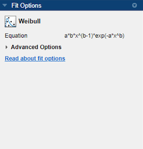
There are no fit settings to configure in the Fit Options pane.
Optionally, in the Advanced Options section, specify coefficient starting values and constraint bounds, or change algorithm settings. The app calculates random start points for Weibull fits, defined on the interval [0 1]. You can override the start points and specify your own values in the Fit Options pane.
For more information on the settings, see Coefficient Constraints: Specify Bounds and Optimized Start Points.
Selecting a Weibull Fit at the Command Line
Specify the model type weibull.
For example, to load some example data measuring blood concentration of a compound against time, and fit and plot a Weibull model specifying a start point:
time = [ 0.1;   0.1;   0.3;   0.3;   1.3;   1.7;   2.1;...
   2.6;   3.9;   3.9; ...
         5.1;   5.6;   6.2;   6.4;   7.7;   8.1;   8.2;...
   8.9;   9.0;   9.5; ...
         9.6;  10.2;  10.3;  10.8;  11.2;  11.2;  11.2;...
  11.7;  12.1;  12.3; ...
        12.3;  13.1;  13.2;  13.4;  13.7;  14.0;  14.3;...
  15.4;  16.1;  16.1; ...
        16.4;  16.4;  16.7;  16.7;  17.5;  17.6;  18.1;...
  18.5;  19.3;  19.7;];
conc = [0.01;  0.08;  0.13;  0.16;  0.55;  0.90;  1.11;...
  1.62;  1.79;  1.59; ...
        1.83;  1.68;  2.09;  2.17;  2.66;  2.08;  2.26;...
  1.65;  1.70;  2.39; ...
        2.08;  2.02;  1.65;  1.96;  1.91;  1.30;  1.62;...
  1.57;  1.32;  1.56; ...
        1.36;  1.05;  1.29;  1.32;  1.20;  1.10;  0.88;...
  0.63;  0.69;  0.69; ...
        0.49;  0.53;  0.42;  0.48;  0.41;  0.27;  0.36;...
  0.33;  0.17;  0.20;];

f=fit(time, conc/25, 'Weibull', ...
'StartPoint', [0.01, 2] )
plot(f,time,conc/25, 'o');
If you want to modify fit options such as coefficient starting values and
constraint bounds appropriate for your data, or change algorithm settings,
see the table of additional properties with
NonlinearLeastSquares on the fitoptions reference
page.
Appropriate start point values and scaling conc/25 for
the two-parameter Weibull model were calculated by fitting a 3 parameter
Weibull model using this custom
equation:
f=fit(time, conc, ' c*a*b*x^(b-1)*exp(-a*x^b)', 'StartPoint', [0.01, 2, 5] )

f =
     General model:
     f(x) = c*a*b*x^(b-1)*exp(-a*x^b)
     Coefficients (with 95% confidence bounds):
       a =    0.009854  (0.007465, 0.01224)
       b =       2.003  (1.895, 2.11)
       c =       25.65  (24.42, 26.89)
See Also
Apps
Functions
fit|fittype|fitoptions