曲線近似の評価
この例では、曲線近似を扱う方法を示します。
データの読み込みと多項式曲線による近似
load census
curvefit = fit(cdate,pop,'poly3','normalize','on')
curvefit =
     Linear model Poly3:
     curvefit(x) = p1*x^3 + p2*x^2 + p3*x + p4
       where x is normalized by mean 1890 and std 62.05
     Coefficients (with 95% confidence bounds):
       p1 =       0.921  (-0.9743, 2.816)
       p2 =       25.18  (23.57, 26.79)
       p3 =       73.86  (70.33, 77.39)
       p4 =       61.74  (59.69, 63.8)
出力には、近似モデル方程式、近似係数、近似係数の信頼限界が表示されます。
近似、データ、残差および予測限界のプロット
plot(curvefit,cdate,pop)

近似の残差をプロットします。
plot(curvefit,cdate,pop,'Residuals')
近似の予測限界をプロットします。
plot(curvefit,cdate,pop,'predfunc')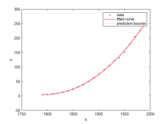
指定した点での近似の評価
x に値を指定し、y = fittedmodel(x) の形式を使用すると、特定の点で近似を評価できます。
curvefit(1991)
ans =
252.6690
多数の点での近似値の評価
モデルを値のベクトルについて評価して 2050 年まで外挿します。
xi = (2000:10:2050).';
curvefit(xi)
ans = 6×1

  276.9632
  305.4420
  335.5066
  367.1802
  400.4859
  435.4468
それらの値の予測限界を取得します。
ci = predint(curvefit,xi)
ci = 6×2

  267.8589  286.0674
  294.3070  316.5770
  321.5924  349.4208
  349.7275  384.6329
  378.7255  422.2462
  408.5919  462.3017
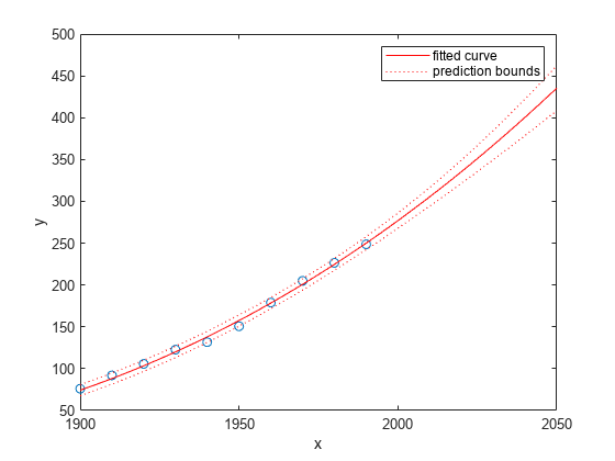
外挿された近似範囲にわたって近似と予測区間をプロットします。既定の設定では、近似はデータの範囲全体についてプロットされます。近似から外挿された値を確認するには、近似をプロットする前に座標軸の x 軸範囲の上限を 2050 に設定します。予測区間をプロットするには、プロット タイプとして predobs または predfun を使用します。
plot(cdate,pop,'o')
xlim([1900,2050])
hold on
plot(curvefit,'predobs')
hold off
モデル方程式の取得
近似名を入力し、モデル方程式、近似係数、近似係数の信頼限界を表示します。
curvefit
curvefit =
     Linear model Poly3:
     curvefit(x) = p1*x^3 + p2*x^2 + p3*x + p4
       where x is normalized by mean 1890 and std 62.05
     Coefficients (with 95% confidence bounds):
       p1 =       0.921  (-0.9743, 2.816)
       p2 =       25.18  (23.57, 26.79)
       p3 =       73.86  (70.33, 77.39)
       p4 =       61.74  (59.69, 63.8)
モデル方程式のみを取得するには formula を使用します。
formula(curvefit)
ans =
'p1*x^3 + p2*x^2 + p3*x + p4'
係数の名前と値の取得
名前で係数を指定します。
p1 = curvefit.p1
p1 =
0.9210
p2 = curvefit.p2
p2 =
25.1834
すべての係数名を取得します。近似方程式 (f(x) = p1*x^3+... など) を確認し、各係数のモデル項を調べます。
coeffnames(curvefit)
ans = 4×1 cell
    {'p1'}
    {'p2'}
    {'p3'}
    {'p4'}
すべての係数値を取得します。
coeffvalues(curvefit)
ans = 1×4

    0.9210   25.1834   73.8598   61.7444
係数の信頼限界の取得
係数の信頼限界を使用すると、近似の評価と比較に役立ちます。係数の信頼限界によって係数の精度が決まります。範囲の間隔が広いほど、不確定性が高いことを示しています。線形係数の範囲がゼロと交差する場合、これらの係数がゼロではないという確信をもてないことを意味します。あるモデル項の係数がゼロの場合、その係数は近似に寄与していません。
confint(curvefit)
ans = 2×4

   -0.9743   23.5736   70.3308   59.6907
    2.8163   26.7931   77.3888   63.7981
適合度の統計量の検証
適合度の統計量をコマンド ラインで取得するには、以下のいずれかを行います。
曲線フィッター アプリを開きます。[曲線フィッター] タブの [エクスポート] セクションで [エクスポート] をクリックし、[ワークスペースにエクスポート] を選択して近似と適合度をワークスペースにエクスポートします。
関数
fitを使用してgof出力引数を指定。
gof と出力引数を指定して近似を再作成し、適合度の統計量と近似アルゴリズム情報を取得します。
[curvefit,gof,output] = fit(cdate,pop,'poly3','normalize','on')
curvefit =
     Linear model Poly3:
     curvefit(x) = p1*x^3 + p2*x^2 + p3*x + p4
       where x is normalized by mean 1890 and std 62.05
     Coefficients (with 95% confidence bounds):
       p1 =       0.921  (-0.9743, 2.816)
       p2 =       25.18  (23.57, 26.79)
       p3 =       73.86  (70.33, 77.39)
       p4 =       61.74  (59.69, 63.8)
gof = struct with fields:
           sse: 149.7687
       rsquare: 0.9988
           dfe: 17
    adjrsquare: 0.9986
          rmse: 2.9682
output = struct with fields:
        numobs: 21
      numparam: 4
     residuals: [21×1 double]
      Jacobian: [21×4 double]
      exitflag: 1
     algorithm: 'QR factorization and solve'
    iterations: 1
残差のヒストグラムをプロットし、おおよそ正規分布に従っていることを確認します。
histogram(output.residuals,10);

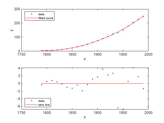
近似、データおよび残差のプロット
figure;
plot(curvefit,cdate,pop,'fit','residuals');
legend Location SouthWest;
メソッドの確認
この近似で使用できるすべてのメソッドを一覧表示します。
methods(curvefit)
Methods for class cfit:

argnames       category       cfit           coeffnames     coeffvalues    confint        dependnames    differentiate  feval          fitoptions     formula        indepnames     integrate      islinear       numargs        numcoeffs      plot           predint        probnames      probvalues     setoptions     type
近似メソッドの使用方法の詳細については、cfitを参照してください。