earthSurfacePermittivity
地表材料の誘電率と伝導率
構文
説明
earthSurfacePermittivity 関数は、地表材料の実数の比誘電率と伝導率、ならびに複素比誘電率を計算します。計算は、国際電気通信連合勧告 (ITU-R) P.527-5 ~ ITU-R P.527-6 [1]に記載されているメソッドと方程式に基づいています。関数 earthSurfacePermittivity には、指定された表面材料に関連する特性を考慮してさまざまな構文が用意されています。
水
[ は、指定された周波数と温度における純水の実数の比誘電率と伝導率、ならびに複素比誘電率を計算します。epsilon,sigma,complexepsilon] = earthSurfacePermittivity("pure-water",fc,temp)
氷
[ は、指定された周波数と温度における不純物がない氷の実数の比誘電率と伝導率、ならびに複素比誘電率を計算します。epsilon,sigma,complexepsilon] = earthSurfacePermittivity("pure-ice",fc,temp)
[ は、指定された周波数と液状水分体積分率における濡れた氷の実数の比誘電率と伝導率、ならびに複素比誘電率を計算します。epsilon,sigma,complexepsilon] = earthSurfacePermittivity("wet-ice",fc,liqfrac)
雪
土壌
[ は、指定された周波数、温度、砂体積率、粘土体積率、比重、および体積含水率における土壌の実数の比誘電率と伝導率、ならびに複素比誘電率を計算します。この構文は、近似式を使用して土壌のかさ密度を計算します。 epsilon,sigma,complexepsilon] = earthSurfacePermittivity("soil",fc,temp,sandpercent,claypercent,sg,vwc)
[ は、前の構文の入力引数に加えて土壌のかさ密度を指定します。epsilon,sigma,complexepsilon] = earthSurfacePermittivity("soil",fc,temp,sandpercent,claypercent,sg,vwc,bulkdensity)
例
純水と海水の実数の比誘電率と伝導率を比較します。
搬送波周波数を 9 GHz として指定します。水の温度を 30℃として指定します。
fc = 9e9; % Hz
temp = 30; % °C
純水と海水の実数の比誘電率と伝導率を計算します。海水の塩分濃度を 35 g/kg として指定します。
[epsilon_pure,sigma_pure] = earthSurfacePermittivity("pure-water",fc,temp);
[epsilon_sea,sigma_sea] = earthSurfacePermittivity("sea-water",fc,temp,35);
実数の比誘電率の値を比較します。
disp("Real relative permittivity of pure water: " + epsilon_pure)Real relative permittivity of pure water: 66.1457
disp("Real relative permittivity of sea water: " + epsilon_sea)Real relative permittivity of sea water: 64.9968
伝導率の値を比較します。
disp("Conductivity of pure water: " + sigma_pure)Conductivity of pure water: 12.6445
disp("Conductivity of sea water: " + sigma_sea)Conductivity of sea water: 13.183
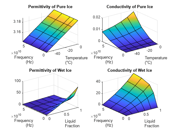
温度が異なる不純物がない氷、および液状水分量が異なる濡れた氷について、実数の比誘電率と伝導率を比較します。
ベクトルを使用して、周波数、液状水分体積分率、および温度の値を指定します。ベクトルを複製し、これらの値から成るグリッドを作成します。
freq0 = [0 10 20 40 60]*1e9;
freq = repmat(freq0,6,1);

liqfrac0 = 0:0.2:1;
liqfrac = repmat(liqfrac0',1,5);

temp0 = -50:10:0;
temp = repmat(temp0',1,5);
周波数と温度の各値について、不純物がない氷の誘電率と伝導率を計算します。関数 arrayfun を使用して、グリッド化された入力の各要素に関数 earthSurfacePermittivity を適用します。
[epsilon_pure,sigma_pure] = arrayfun(@(x,y) ...
    earthSurfacePermittivity("pure-ice",x,y),freq,temp);
周波数と液状水分体積分率の各値について、濡れた氷の誘電率と伝導率を計算します。
[epsilon_wet,sigma_wet] = arrayfun(@(x,y) ...
    earthSurfacePermittivity("wet-ice",x,y),freq,liqfrac);
複数の表面のプロットを使用して結果を表示します。タイル表示チャート レイアウトを使用してプロットを整理します。
figure
tiledlayout(2,2)

nexttile
surf(temp,freq,epsilon_pure,FaceColor="interp")
title("Permittivity of Pure Ice")
xlabel(["Temperature","(°C)"])
ylabel(["Frequency","(Hz)"])

nexttile
surf(temp,freq,sigma_pure,FaceColor="interp")
title("Conductivity of Pure Ice")
xlabel(["Temperature","(°C)"])
ylabel(["Frequency","(Hz)"])

nexttile
surf(liqfrac,freq,epsilon_wet,FaceColor="interp")
title("Permittivity of Wet Ice")
xlabel(["Liquid","Fraction"])
ylabel(["Frequency","(Hz)"])

nexttile
surf(liqfrac,freq,sigma_wet,FaceColor="interp")
title("Conductivity of Wet Ice")
xlabel(["Liquid","Fraction"])
ylabel(["Frequency","(Hz)"])
いくつかの土壌混合物の実数の比誘電率と伝導率を計算します。
搬送波周波数、土壌の温度、および土壌の体積含水率を指定します。
fc = 28e9; % Hz
temp = 23; % °C
vwc = 0.5;
ITU-R P.527-6 では、さまざまなタイプの土壌のテキスト分類が定義されています。これらの分類は、土壌に含まれる砂、粘土、およびシルトの割合によって決まります。ITU-R P.527-6 の Table 2 の値を使用して、砂壌土、壌土、シルト質壌土、シルト質粘土に含まれる砂と粘土の代表的な割合を指定します。これらの値を使用して、シルトの割合を計算します。
soilType = ["Sandy Loam","Loam","Silty Loam","Silty Clay"]';
percentSand = [51.52 41.96 30.63 5.02]';
percentClay = [13.42 8.53 13.48 47.38]';
percentSilt = 100 - (percentSand + percentClay);
ITU-R P.527-6 の Table 2 の値を使用して、砂壌土、壌土、シルト質壌土、シルト質粘土の比重とかさ密度の代表的な値を指定します。
sg = [2.66 2.70 2.59 2.56]';
bulkdensity = [1.6006 1.5781 1.5750 1.4758]'; % g/cm^3
変数を table に収集します。
varNames1 = ["Soil Textual Classification","Sand (%)","Clay (%)", ...
    "Silt (%)","Specific Gravity","Bulk Density"]';
T1 = table(soilType,percentSand,percentClay,percentSilt, ...
    sg,bulkdensity,VariableNames=varNames1)
T1=4×6 table
    Soil Textual Classification    Sand (%)    Clay (%)    Silt (%)    Specific Gravity    Bulk Density
    ___________________________    ________    ________    ________    ________________    ____________

           "Sandy Loam"             51.52       13.42       35.06            2.66             1.6006
           "Loam"                   41.96        8.53       49.51             2.7             1.5781
           "Silty Loam"             30.63       13.48       55.89            2.59              1.575
           "Silty Clay"              5.02       47.38        47.6            2.56             1.4758
各タイプの土壌の実数の比誘電率と伝導率を計算します。関数 arrayfun を使用して、入力の各要素に関数 earthSurfacePermittivity を適用します。
[Permittivity,Conductivity] = arrayfun(@(w,x,y,z) ...
    earthSurfacePermittivity("soil",fc,temp,w,x,y,vwc,z), ...
    percentSand,percentClay,sg,bulkdensity);
結果を table に収集します。
varNames2 = ["Soil Textual Classification", ...
    "Real Relative Permittivity","Conductivity"]';
T2 = table(soilType,Permittivity,Conductivity,VariableNames=varNames2)
T2=4×3 table
    Soil Textual Classification    Real Relative Permittivity    Conductivity
    ___________________________    __________________________    ____________

           "Sandy Loam"                      15.281                   18.2
           "Loam"                            14.563                 16.998
           "Silty Loam"                      13.965                 16.011
           "Silty Clay"                      12.861                 14.647
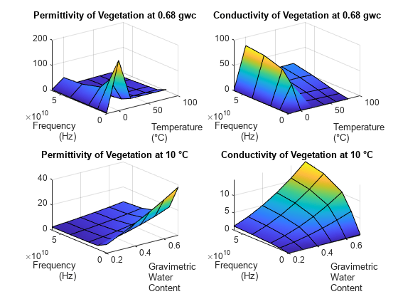
植生の実数の比誘電率と伝導率を計算します。さまざまな周波数、温度、重量含水率の値について、誘電率と伝導率を比較します。
1 つの周波数、温度、および重量含水率における計算
搬送波周波数を 9 GHz、植生の温度を 23℃、植生の重量含水率を 0.68 として指定します。植生の実数の比誘電率と伝導率を計算します。
fc = 10e9; % Hz
temp  = 23; % °C
gwc = 0.68;

[epsilon_veg,sigma_veg] = earthSurfacePermittivity("vegetation",fc,temp,gwc)
epsilon_veg =
20.5757
sigma_veg =
4.9320
複数の周波数、温度、および重量含水率の比較
さまざまな周波数、温度、重量含水率の値について、実数の比誘電率と伝導率を比較します。
ベクトルを使用して、周波数、温度、および重量含水率を指定します。ベクトルを複製し、これらの値から成るグリッドを作成します。
fc0 = [0 10 20 40 60]*1e9;
temp0 = -20:20:80;
gwc0 = 0.2:0.1:0.7;

fc = repmat(fc0,6,1);
temp = repmat(temp0',1,5);
gwc = repmat(gwc0',1,5);
周波数と温度の各値について、植生の誘電率と伝導率を計算します。重量含水率の値には 0.68 を使用します。関数 arrayfun を使用して、グリッド化された入力の各要素に関数 earthSurfacePermittivity を適用します。
[epsilon_veg_gwc,sigma_veg_gwc] = arrayfun(@(x,y) ...
    earthSurfacePermittivity("vegetation",x,y,0.68),fc,temp);
周波数と重量含水率の各値について、植生の誘電率と伝導率を計算します。温度の値には 10℃を使用します。
[epsilon_veg_tmp,sigma_veg_tmp] = arrayfun(@(x,z) ...
    earthSurfacePermittivity("vegetation",x,10,z),fc,gwc);
複数の表面のプロットを使用して結果を表示します。タイル表示チャート レイアウトを使用してプロットを整理します。
figure
tiledlayout(2,2)

nexttile
surf(temp,fc,epsilon_veg_gwc,FaceColor="interp")
title("Permittivity of Vegetation at 0.68 gwc")
xlabel(["Temperature","(°C)"])
ylabel(["Frequency","(Hz)"])

nexttile
surf(temp,fc,sigma_veg_gwc,"FaceColor","interp")
title("Conductivity of Vegetation at 0.68 gwc")
xlabel(["Temperature","(°C)"])
ylabel(["Frequency","(Hz)"])

nexttile
surf(gwc,fc,epsilon_veg_tmp,"FaceColor","interp")
title("Permittivity of Vegetation at 10 °C")
xlabel(["Gravimetric","Water","Content"])
ylabel(["Frequency","(Hz)"])

nexttile
surf(gwc,fc,sigma_veg_tmp,"FaceColor","interp")
title("Conductivity of Vegetation at 10 °C")
xlabel(["Gravimetric","Water","Content"])
ylabel(["Frequency","(Hz)"])
入力引数
出力引数
詳細
参照
[1] International Telecommunications Union Radiocommunication Sector. Electrical Characteristics of the Surface of the Earth. Recommendation P.527. ITU-R, approved September 27, 2021. https://www.itu.int/rec/R-REC-P.527/en.
[2] Mohr, Peter J., Eite Tiesinga, David B. Newell, and Barry N. Taylor. “Codata Internationally Recommended 2022 Values of the Fundamental Physical Constants.” NIST, May 8, 2024. https://www.nist.gov/publications/codata-internationally-recommended-2022-values-fundamental-physical-constants.