結果:

0 - 1 / 1

General

Athanasios Paraskevopoulos
最後のアクティビティ: 2024 年 3 月 17 日

Helmholtz problem in circular disk

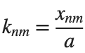
The following expression

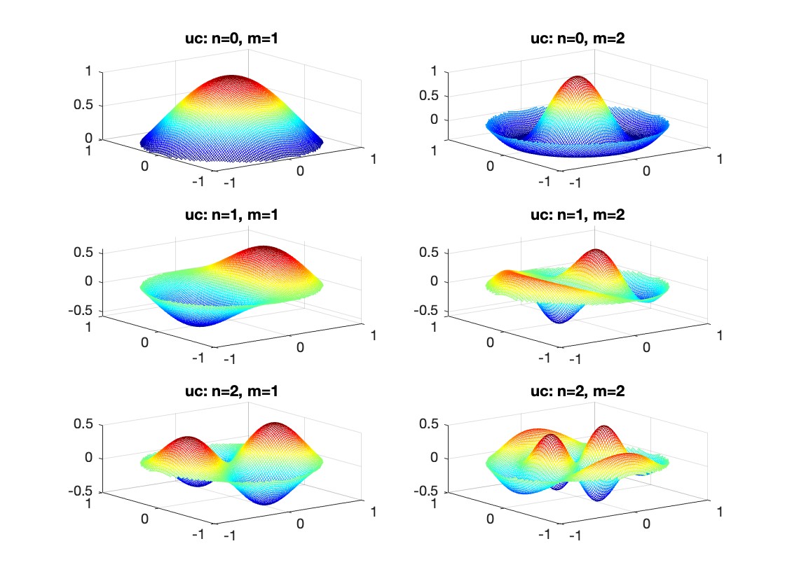
gives the solution for the Helmholtz problem. On the circular disc with center 0 and radius a. For

the plot in 3-dimensional graphics of the solutions on Matlab for

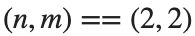and then calculate some eigenfunctions with the following expression.

It could be better to separate functions with

and

as follows

diska = 1;  % Radius of the disk
mmax = 2;   % Maximum value of m
nmax = 2;   % Maximum value of n
% Function to find the k-th zero of the n-th Bessel function
% This function uses a more accurate method for initial guess
besselzero = @(n, k) fzero(@(x) besselj(n, x), [(k-(n==0))*pi, (k+1-(n==0))*pi]);
% Define the eigenvalue k[m, n] based on the zeros of the Bessel function
k = @(m, n) besselzero(n, m);
% Define the functions uc and us using Bessel functions
% These functions represent the radial part of the solution
uc = @(r, t, m, n) cos(n * t) .* besselj(n, k(m, n) * r);
us = @(r, t, m, n) sin(n * t) .* besselj(n, k(m, n) * r);
% Generate data for demonstration
data = zeros(5, 3);
for m = 1:5
    for n = 0:2
        data(m, n+1) = k(m, n);  % Storing the eigenvalues
    end
end
% Display the data
disp(data);
% Plotting all in one figure
figure;
plotIndex = 1;
for n = 0:nmax
    for m = 1:mmax
        subplot(nmax + 1, mmax, plotIndex);
        [X, Y] = meshgrid(linspace(-diska, diska, 100), linspace(-diska, diska, 100));
        R = sqrt(X.^2 + Y.^2);
        T = atan2(Y, X);
        Z = uc(R, T, m, n);  % Using uc for plotting
        % Ensure the plot is only within the disk
        Z(R > diska) = NaN;
        mesh(X, Y, Z);
        title(sprintf('uc: n=%d, m=%d', n, m));
        colormap('jet');
        plotIndex = plotIndex + 1;
    end
end

0 - 1 / 1