ans =
結果:
I'd like to share some tips about the 2024 mini hack contest, specifically related to audio:
- First (and most important), credit your source: unless you are composing your own audio, I think it's important to give credit to the original sources. It is a little sad to see several contributions with an empty line:
'Cite your audio source here (if applicable):'
- A great place to get royalty-free and high-quality music and audio (among other media) is https://pixabay.com. Be sure to check it out! I used one of their audio clips in my submission EKG pulse
- The right music can enhance the overall experience of your animation. Sometimes getting the animation to match the music beat can be hard. I suggest you try the other way around: get your music/sound effects to match the animation rhythm with a little editing. A free audio editor with many capabilities (more than enough for this contest, I think) is https://www.audacityteam.org/
- Choose a 4-second audio clip with a consistent tempo and seamless loop points, ensuring it complements your animation's mood and loops smoothly over 12 seconds without abrupt changes.
I think that when the right music is paired with the right animation, it can create a more impactful experience.
Well, this is my first time to participate in such community competitions and guess what, I've gone for 4 submissions so far (Feels Great!!)
So I wanna share some tricks that I followed for my first submission named Happy Shaping' ( Go Check it out!!):
1. Dynamic Background Color Change:
- Technique: The background color of the figure window is gradually changed using sine and cosine functions.
- Reason: These trigonometric functions (sin and cos) create smooth, oscillating transitions over time, which gives a fluid effect to the background's color shift.
- Implementation:
Color = [0.1 + 0.5*abs(sin(f/10)), 0.1 + 0.5*abs(cos(f/15)), 0.9 -
0.5*abs(sin(f/20))];
- Benefit: This introduces a smooth, visually appealing animation effect.
2. Smooth Object Motion Using Sine and Cosine:
- Technique: The position and shape of objects are based on trigonometric functions.
- Reason: Using sin(t) and cos(t) ensures that the movement is circular or elliptical, creating continuous and natural motion in animations.
- Implementation (for object position):
x = 10 * cos(t * 2 * pi) * (1 + 0.5 * sin(t * pi));
y = 10 * sin(t * 2 * pi) * (1 + 0.5 * cos(t * pi));
- Benefit: Circular and smooth motions are pleasing and easily controlled by tweaking the frequency and phase of sine/cosine functions.
3. Polygon Shape Changing Over Time:
- Technique: The number of sides of the polygon (sides) changes dynamically based on t.
- Reason: It creates variation in shape, maintaining user interest as the shape transitions from a triangle to a hexagon.
- Implementation:
sides = 3 + round(3 * abs(sin(t)));
- Benefit: This provides dynamic shape transitions over time, keeping the animation non-static.
4. Use of the fill Function for Color-Filled Shapes:
- Technique: The fill function is used to draw a polygon with smoothly changing colors.
- Reason: Filling polygons with varying colors based on time (t) allows for continuous color transitions, adding more complexity to the animation.
- Implementation:
fill(xp, yp, c, 'EdgeColor', 'none');
- Benefit: Combining both color changes and shape changes enhances the visual impact.
5. Consistent Use of hold on and hold off:
- Technique: hold on allows multiple graphic objects to be drawn on the same axes without clearing previous objects.
- Reason: This is crucial for drawing multiple elements (like polygons, circles, and lines) on the same figure.
- Benefit: It helps manage and layer different graphical elements effectively within the same frame.
6. Use of rectangle for a Smooth Ball Motion:
- Technique: The ball's motion is defined by rectangle with a Curvature of [1, 1] to make it circular.
- Reason: Using the rectangle function simplifies the process of drawing a filled circle, and controlling its position and size is intuitive.
- Benefit: It provides a straightforward way to animate circular objects within the plot.
7. Animating the Connection Line:
- Technique: A white dashed line (w--) is drawn between the polygon and the moving ball to show a connection between these objects.
- Reason: This adds interactivity to the scene, as it gives the impression that the polygon and the ball are related or connected in some way.
- Implementation:
plot([x bx], [y by], 'w--', 'LineWidth', 2);
- Benefit: A dynamic element that adds depth and narrative to the animation, guiding the viewer’s attention.
8. Frame Synchronization with Time (f and t):
- Technique: The variable f is used as a frame number, while t = f / 24 creates a link between frame and time.
- Reason: Ensuring smooth and continuous transitions in the animation over time is critical, so f acts as the control for time-based changes in shape, color, and position.
- Benefit: This makes it easy to manage frame rates and time-based updates for the animation.
If you like them, please feel free to use them for free.
function drawframe(f)
% Create a figure
figure;
hold on;
axis equal;
axis off;
% Draw the roads
rectangle('Position', [0, 0, 2, 30], 'FaceColor', [0.5 0.5 0.5]); % Left road
rectangle('Position', [2, 0, 2, 30], 'FaceColor', [0.5 0.5 0.5]); % Right road
% Draw the traffic light
trafficLightPole = rectangle('Position', [-1, 20, 1, 0.2], 'FaceColor', 'black'); % Pole
redLight = rectangle('Position', [0, 20, 0.5, 1], 'FaceColor', 'red'); % Red light
yellowLight = rectangle('Position', [0.5, 20, 0.5, 1], 'FaceColor', 'black'); % Yellow light
greenLight = rectangle('Position', [1, 20, 0.5, 1], 'FaceColor', 'black'); % Green light
carBody = rectangle('Position', [2.5, 2, 1, 4], 'Curvature', 0.2, 'FaceColor', 'red'); % Body
leftWheel = rectangle('Position', [2.5, 3.0, 0.2, 0.2], 'Curvature', [1, 1], 'FaceColor', 'black'); % Left wheel
rightWheel = rectangle('Position', [3.3, 3.0, 0.2, 0.2], 'Curvature', [1, 1], 'FaceColor', 'black'); % Right wheel
leftFrontWheel = rectangle('Position', [2.5, 5.0, 0.2, 0.2], 'Curvature', [1, 1], 'FaceColor', 'black'); % Left wheel
rightFrontWheel = rectangle('Position', [3.3, 5.0, 0.2, 0.2], 'Curvature', [1, 1], 'FaceColor', 'black'); % Right wheel
% Set limits
xlim([-1, 8]);
ylim([-1, 35]);
% Animation parameters
carSpeed = 0.5; % Speed of the car
carPosition = 2; % Initial car position
stopPosition = 15; % Position to stop at the traffic light
isStopped = false; % Car is not stopped initially
%Animation loop
for t = 1:100
% Update traffic light: Red for 40 frames, yellow for 10 frames Green for 40 frames
if t <= 40
% Red light on, yellow and green off
set(redLight, 'FaceColor', 'red');
set(yellowLight, 'FaceColor', 'black');
set(greenLight, 'FaceColor', 'black');
elseif t > 40 && t <= 50
% Change to green light
set(redLight, 'FaceColor', 'black');
set(yellowLight, 'FaceColor', 'yellow');
set(greenLight, 'FaceColor', 'black');
else
% Back to red light
set(redLight, 'FaceColor', 'black');
set(yellowLight, 'FaceColor', 'black');
set(greenLight, 'FaceColor', 'green');
isStopped = false; % Allow car to move
end
%Move the car
if ~isStopped
carPosition = carPosition + carSpeed; % Move forward
if carPosition < stopPosition
%do nothing
else
isStopped = true;
end
else
% Gradually stop the car when red
if carPosition > stopPosition
carPosition = carPosition + carSpeed*(1-t/50); % Move backward until it reaches the stop position
end
end
if carPosition >= 25
carPosition = 25;
end
% Update car position
% set(carBody, 'Position', [carPosition, 2, 1, 0.5]);
set(carBody, 'Position', [2.5, carPosition, 1, 4]);
%set(carWindow, 'Position', [carPosition + 0.2, 2.4, 0.6, 0.2]);
%set(leftWheel, 'Position', [carPosition, 1.5, 0.2, 0.2]);
set(leftWheel, 'Position', [2.5, carPosition+1, 0.2, 0.2]);
% set(rightWheel, 'Position', [carPosition + 0.8, 1.5, 0.2, 0.2]);
set(rightWheel, 'Position', [3.3, carPosition+1, 0.2, 0.2]);
set(leftFrontWheel, 'Position', [2.5, carPosition+3, 0.2, 0.2]);
set(rightFrontWheel, 'Position', [3.3, carPosition+3, 0.2, 0.2]);
% Pause to control animation speed
pause(0.01);
end
hold off;
Try to install MATLAB2024a on Ubuntu24.04. In the image below, the button indicated by the green arrow is clickable, while the button indicated by the red arrow are unclickable, and input field where text cannot be entered, preventing the installation.

Do you use MATLAB Online for teaching? MATLAB Online lets students run MATLAB without having to install the software on the computer. All you need is a web browser and an internet connection.
I would love to hear comments and experiences of using MATLAB Online.
Let's say you have a chance to ask the MATLAB leadership team any question. What would you ask them?
Hi, My data send to thingspeak is not received/updated for the last 6 hours on the charts and dials. All worked well till about 6 hour ago. I am using Node-red and the API Url: https://thingspeak.com
Any help please?
Greetings Gert
To solve issues around the browsers blocking 3p cookies and having different behavior across different browsers, the ThingSpeak website is now served from https://thingspeak.mathworks.com. There are no changes required from devices or users. Just log in and use the service as you always did.
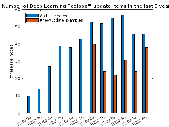
What is the side-effect of counting the number of Deep Learning Toolbox™ updates in the last 5 years? The industry has slowly stabilised and matured, so updates have slowed down in the last 1 year, and there has been no exponential growth.Is it correct to assume that? Let's see what you think!
releaseNumNames = "R"+string(2019:2024)+["a";"b"];
releaseNumNames = releaseNumNames(:);
numReleaseNotes = [10,14,27,39,38,43,53,52,55,57,46,46];
exampleNums = [nan,nan,nan,nan,nan,nan,40,24,22,31,24,38];
bar(releaseNumNames,[numReleaseNotes;exampleNums]')
legend(["#release notes","#new/update examples"],Location="northwest")
title("Number of Deep Learning Toolbox™ update items in the last 5 years")
ylabel("#release notes")
I left the code unchanged, modifying only secrets.h.
I am using an ESP32-WROOM -32U
Connection to network succeeds, but ThingSpeak.writeFields fails every time, with HTTP error code 400.
The sketch I am really trying to use is loosely based on this example, accesses Time and Weather info with no problems, but ThingSpeak.writeFields fails with HTTP error code 301.
This is my first attempt to use ThingSpeak.
Is this example sketch still valid, or must I look elsewhere? Suggestions please.
How can I mechanically couple synchronous reluctance motor from simscape electrical electromechanical library and dc generator from specialized power system library
Hi everyone,
I'm working on a school project where I need to send sensor data from my Arduino to a Power BI REST API using ThingsHTTP. I've been trying to get this to work, but I'm running into errors like this:
{"error":{"code":"InvalidRequest","message":"Error parsing request for dataset sobe_wowvirtualserver|a7b68fb5-533b-471f-a5da-3bdd6746ee16: Conversion error on column '<pi>pH</pi>': <pi>Input string was not in a correct format.</pi>"}}
I'm a beginner with this, and I'm not sure what I'm doing wrong. What steps should I take to resolve this issue? Also, does anyone know the correct format for an HTTP request body when sending dynamic sensor data?
This is the body format I'm trying to send to Power BI:
[
{
"pH": 98.6,
"TDS": 98.6,
"turbidity": 98.6,
"temperature": 98.6
}
]
Any advice on how to construct the HTTP body with values that change over time would be greatly appreciated! Thanks in advance!"
hope this message finds you well. I am currently working on a project involving the design and numerical simulation of metalenses using Zemax and MATLAB. The design phase involves saving phase data from the Zemax simulation, which is later used in a numerical script to generate the metalens in MATLAB.
I have a MATLAB file that contains the phase data saved from Zemax, but I am unsure of the specific method or format used to extract and save the data from Zemax. The phase data I currently have in MATLAB is as follows:
- Phase matrix: 571 x 571 (double)
- X data: 571 x 1 (double)
- Y data: 571 x 1 (double)
Could you please provide guidance on:
- How this phase data was likely saved from Zemax into MATLAB?
- What steps or scripts were used to extract this information from the design, particularly the 571 x 571 phase matrix and the corresponding X and Y data?
- Any best practices or tools available in Zemax for exporting such data?
This information will help me reproduce the workflow and proceed with my analysis.
Thank you for your support. I look forward to your guidance.
Best regards,
Zaka

See the attached PDF for a higher resolution
Related blogs posts:
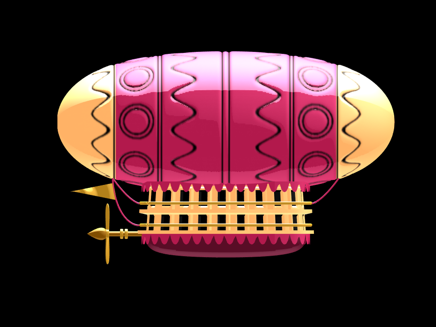
In the spirit of warming up for this year's minihack contest, I'm uploading a walkthrough for how to design an airship using pure Matlab script. This is commented and uncondensed; half of the challenge for the minihacks is how minimize characters. But, maybe it will give people some ideas.
The actual airship design is from one of my favorite original NES games that I played when I was a kid - Little Nemo: The Dream Master. The design comes from the intro of the game when Nemo sees the Slumberland airship leave for Slumberland:
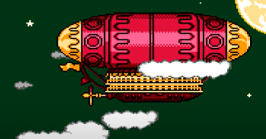
(Snip from a frame of the opening scene in Capcom's game Little Nemo: The Dream Master, showing the Slumberland airship).
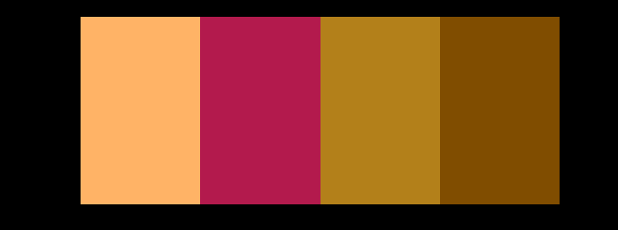
I spent hours playing this game with my two sisters, when we were little. It's fun and tough, but the graphics sparked the imagination. On to the code walkthrough, beginning with the color palette: these four colors are the only colors used for the airship:
c1=cat(3,1,.7,.4); % Cream color
c2=cat(3,.7,.1,.3); % Magenta
c3=cat(3,0.7,.5,.1); % Gold
c4=cat(3,.5,.3,0); % bronze
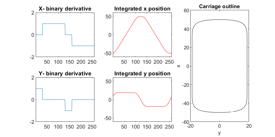
We start with the airship carriage body. We want something rectangular but smoothed on the corners. To do this we are going to start with the separate derivatives of the x and y components, which can be expressed using separate blocks of only three levels: [1, 0, -1]. You could integrate to create a rectangle, but if we smooth the derivatives prior to integrating we will get rounded edges. This is done in the following code:
% Binary components for x & y vectors
z=zeros(1,30);
o=ones(1,100);
% X and y vectors
x=[z,o,z,-o];
y=[1+z,1-o,z-1,1-o];
% Smoother function (fourier / circular)
s=@(x)ifft(fft(x).*conj(fft(hann(45)'/22,260)));
% Integrator function with replication and smoothing to form mesh matrices
u=@(x)repmat(cumsum(s(x)),[30,1]);
% Construct x and y components of carriage with offsets
x3=u(x)-49.35;
y3=u(y)+6.35;
y3 = y3*1.25; % Make it a little fatter
% Add a z-component to make the full set of matrices for creating a 3D
% surface:
z3=linspace(0,1,30)'.*ones(1,260)*30;
z3(14,:)=z3(15,:); % These two lines are for adding platforms
z3(2,:)=z3(3,:); % to the carriage, later.
Plotting x, y, and the top row of the smoothed, integrated, and replicated matrices x3 and y3 gives the following:
We now have the x and y components for a 3D mesh of the carriage, let's make it more interesting by adding a color scheme including doors, and texture for the trim around the doors. Let's also add platforms beneath the doors for passengers to walk on.
Starting with the color values, let's make doors by convolving points in a color-matrix by a door shaped function.
m=0*z3; % Image matrix that will be overlayed on carriage surface
m(7,10:12:end)=1; % Door locations (lower deck)
m(21,10:12:end)=1; % Door locations (upper deck)
drs = ones(9, 5); % Door shape
m=1-conv2(m,ones(9,5),'same'); % Applying
To add the trim, we will convolve matrix "m" (the color matrix) with a square function, and look for values that lie between the extrema. We will use this to create a displacement function that bumps out the -x, and -y values of the carriage surface in intermediary polar coordinate format.
rm=conv2(m,ones(5)/25,'same'); % Smoothing the door function
rm(~m)=0; % Preserving only the region around the doors
rds=0*m; % Radial displacement function
rds(rm<1&rm>0)=1; % Preserving region around doors
rds(m==0)=0;
rds(13:14,:)=6; % Adding walkways
rds(1:2,:)=6;
% Apply radial displacement function
[th,rd]=cart2pol(x3,y3);
[x3T,y3T]=pol2cart(th,(rd+rds)*.89);
If we plot the color function (m) and radial displacement function (rds) we get the following:
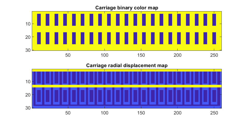
In the upper plot you can see the doors, and in the bottom map you can see the walk way and door trim.
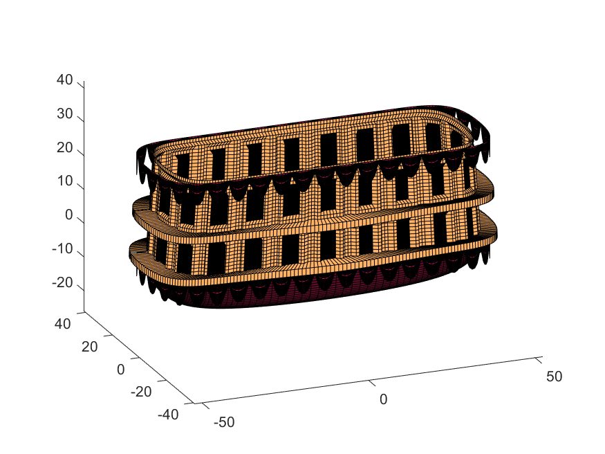
Next, we are going to add some flags draped from the bottom and top of the carriage. We are going to recycle the values in "z3" to do this, by multiplying that matrix with the absolute value of a sine-wave, squished a bit with the soft-clip erf() function.
We add a keel to the airship carriage using a canonical sphere turned on its side, again using the soft-clip erf() function to make it roughly rectangular in x and y, and multiplying with a vector that is half nan's to make the top half transparent.
At this point, since we are beginning the plotting of the ship, we also need to create our hgtransform objects. These allow us to move all of the components of the airship in unison, and also link objects with pivot points to the airship, such as the propeller.
% Now we need some flags extending around the top and bottom of the
% carriage. We can do this my multiplying the height function (z3) with the
% absolute value of a sine-wave, rounded with a compression function
% (erf() in this case);
g=-z3.*erf(abs(sin(linspace(0,40*pi,260))))/4; % Flags
% Also going to add a slight taper to the carriage... gives it a nice look
tp=linspace(1.05,1,30)';
% Finally, plotting. Plot the carriage with the color-map for the doors in
% the cream color, than the flags in magenta. Attach them both to transform
% objects for movement.
% Set up transform objects. 2 moving parts:
% 1) The airship itself and all sub-components
% 2) The propellor, which attaches to the airship and spins on its axis.
hold on;
P=hgtransform('Parent',gca); % Ship
S=hgtransform('Parent',P); % Prop
surf(x3T.*tp,y3T,z3,c1.*m,'Parent',P);
surf(x3,y3,g,c2.*rd./rd, 'Parent', P);
surf(x3,y3,g+31,c2.*rd./rd, 'Parent', P);
axis equal
% Now add the keel of the airship. Will use a canonical sphere and the
% erf() compression function to square off.
[x,y,z]=sphere(99);
mk=round(linspace(-1,1).^2+.3); % This function makes the top half of the sphere nan's for transparency.
surf(50*erf(1.4*z),15*erf(1.4*y),13*x.*mk./mk-1,.5*c2.*z./z, 'Parent', P);
% The carriage is done. Now we can make the blimp above it.
We haven't adjusted the shading of the image yet, but you can see the design features that have been created:
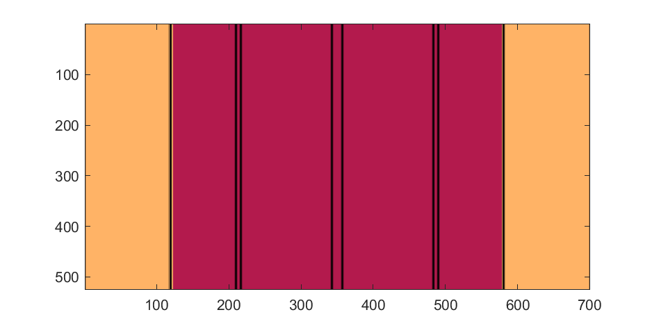
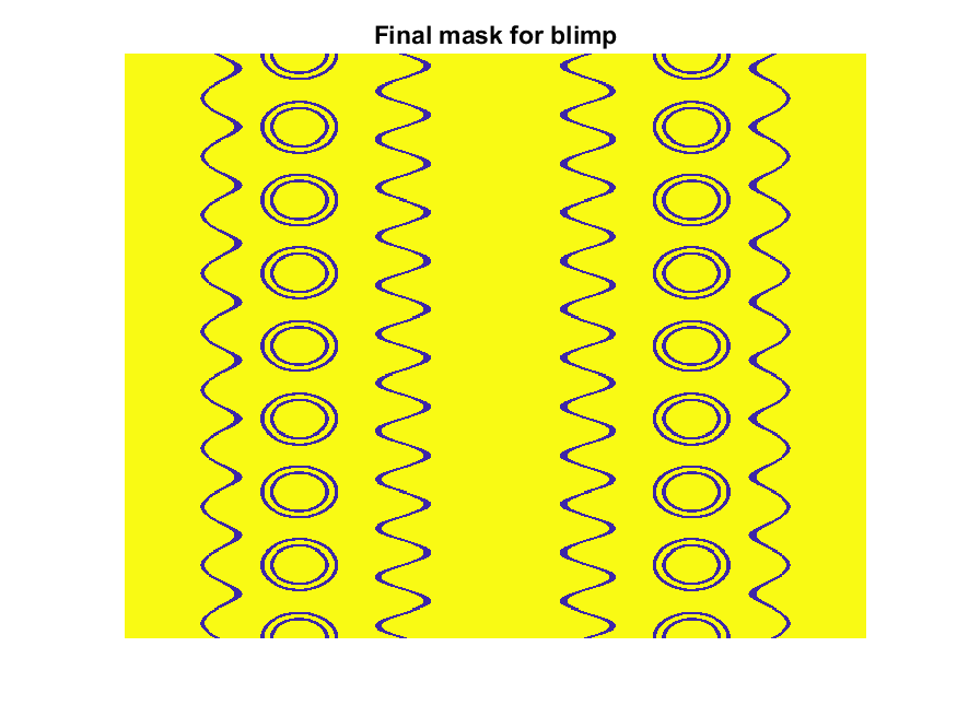
Next, we start working on the blimp. This is going to use a few more vertices & faces. We are going to use a tapered cylinder for this part, and will start by making the overlaid image, which will have 2 colors plus radial rings, circles, and squiggles for ornamentation.
M=525; % Blimp (matrix dimensions)
N=700;
% Assign the blimp the cream and magenta colors
t=122; % Transition point
b=ones(M,N,3); % Blimp color map template
bc=b.*c1; % Blimp color map
bc(:,t+1:end-t,:)=b(:,t+1:end-t,:).*c2;
% Add axial rings around blimp
l=[.17,.3,.31,.49];
l=round([l,1-fliplr(l)]*N); % Mirroring
lnw=ones(1,N); % Mask
lnw(l)=0;
lnw=rescale(conv(lnw,hann(7)','same'));
bc=bc.*lnw;
% Now add squiggles. We're going to do this by making an even function in
% the x-dimension (N, 725) added with a sinusoidal oscillation in the
% y-dimension (M, 500), then thresholding.
r=sin(linspace(0, 2*pi, M)*10)'+(linspace(-1, 1, N).^6-.18)*15;
q=abs(r)>.15;
r=sin(linspace(0, 2*pi, M)*12)'+(abs(linspace(-1, 1, N))-.25)*15;
q=q.*(abs(r)>.15);
% Now add the circles on the blimp. These will be spaced evenly in the
% polar angle dimension around the axis. We will have 9. To make the
% circles, we will create a cone function with a peak at the center of the
% circle, and use thresholding to create a ring of appropriate radius.
hs=[1,.75,.5,.25,0,-.25,-.5,-.75,-1]; % Axial spacing of rings
% Cone generation and ring loop
xy= @(h,s)meshgrid(linspace(-1, 1, N)+s*.53,(linspace(-1, 1, M)+h)*1.15);
w=@(x,y)sqrt(x.^2+y.^2);
for n=1:9
h=hs(n);
[xx,yy]=xy(h,-1);
r1=w(xx,yy);
[xx,yy]=xy(h,1);
r2=w(xx,yy);
b=@(x,y)abs(y-x)>.005;
q=q.*b(.1,r1).*b(.075,r1).*b(.1,r2).*b(.075,r2);
end
The figures below show the color scheme and mask used to apply the squiggles and circles generated in the code above:
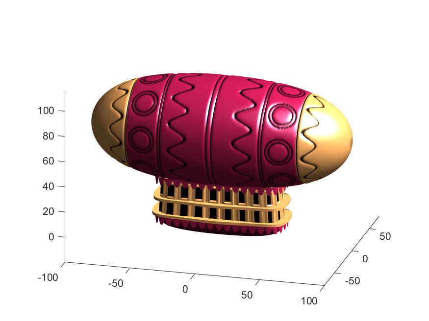
Finally, for the colormap we are going to smooth the binary mask to avoid hard transitions, and use it to to add a "puffy" texture to the blimp shape. This will be done by diffusing the mask iteratively in a loop with a non-linear min() operator.
% 2D convolution function
ff=@(x)circshift(ifft2(fft2(x).*conj(fft2(hann(7)*hann(7)'/9,M,N))),[3,3]);
q=ff(q); % Smooth our mask function
hh=rgb2hsv(q.*bc); % Convert to hsv: we are going to use the value
% component for radial displacement offsets of the
% 3D blimp structure.
rd=hh(:,:,3); % Value component
for n=1:10
rd=min(rd,ff(rd)); % Diffusing the value component for a puffy look
end
rd=(rd+35)/36; % Make displacements effects small
% Now make 3D blimp manifold using "cylinder" canonical shape
[x,y,z]=cylinder(erf(sin(linspace(0,pi,N)).^.5)/4,M-1); % First argument is the blimp taper
[t,r]=cart2pol(x, y);
[x2,y2]=pol2cart(t, r.*rd'); % Applying radial displacment from mask
s=200;
% Plotting the blimp
surf(z'*s-s/2, y2'*s, x2'*s+s/3.9+15, q.*bc,'Parent',P);
Notice that the parent of the blimp surface plot is the same as the carriage (e.g. hgtransform object "P"). Plotting at this point using flat shading and adding some lighting gives the image below:
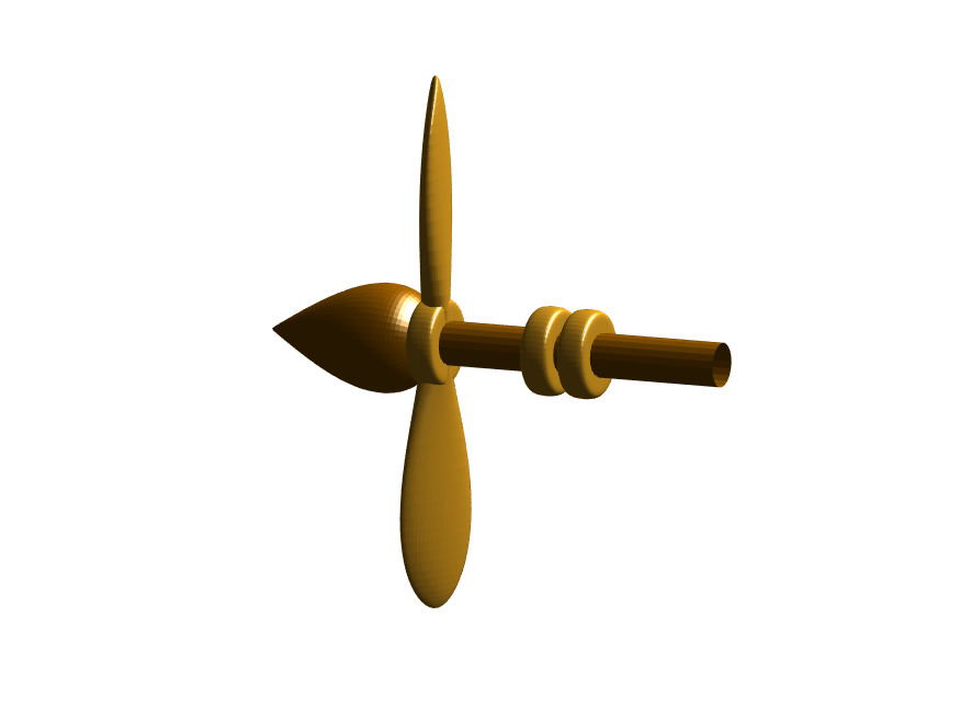
Next, we need to add a propeller so it can move. This will include the creation of a shaft using the cylinder() function. The rest of the pieces (the propeller blades, collars and shaft tip) all use the same canonical sphere with distortions applied using various math functions. Note that when the propeller is made it is linked to hgtransform object "S" rather than "P." This will allow the propeller to rotate, but still be joined to the airship.
% Next, the propeller. First, we start with the shaft. This is a simple
% cylinder. We add an offset variable and a scale variable to move our
% propeller components around, as well.
shx = -70; % This is our x-shifter for components
scl = 3; % Component size scaler
[x,y,z]=cylinder(1, 20); % Canonical cylinder for prop shaft.
p(1)=surf(-scl*(z-1)*7+shx,scl*x/2,scl*y/2,0*x+c4,'Parent',P); % Prop shaft
% Now the propeller. This is going to be made from a distorted sphere.
% The important thing here is that it is linked to the "S" hgtransform
% object, which will allow it to rotate.
[x,y,z]=sphere(50);
a=(-1:.04:1)';
x2=(x.*cos(a)-y/3.*sin(a)).*(abs(sin(a*2))*2+.1);
y2=(x.*sin(a)+y/3.*cos(a));
p(2)=surf(-scl*y2+shx,scl*x2,scl*z*6,0*x+c3,'Parent',S);
% Now for the prop-collars. You can see these on the shaft in the NES
% animation. These will just be made by using the canonical sphere and the
% erf() activation function to square it in the x-dimension.
g=erf(z*3)/3;
r=@(g)surf(-scl*g+shx,scl*x,scl*y,0*x+c3,'Parent',P);
r(g);
r(g-2.8);
r(g-3.7);
% Finally, the prop shaft tip. This will just be the sphere with a
% taper-function applied radially.
t=1.7*cos(0:.026:1.3)'.^2;
p(3)=surf(-(z*2+2)*scl + shx,x.*t*scl,y.*t*scl, 0*x+c4,'Parent',P);
Now for some final details including the ropes to the blimp, a flag hung on one of the ropes, and railings around the walkways so that passengers don't plummet to their doom. This will make use of the ad-hoc "ropeG" function, which takes a 3D vector of points and makes a conforming cylinder around it, so that you get lighting functions etc. that don't work on simple lines. This function is added to the script at the end to do this:
% Rope function for making a 3D curve have thickness, like a rope.
% Inputs:
% - xyz (3D curve vector, M points in 3 x M format)
% - N (Number of radial points in cylinder function around the curve
% - W (Width of the rope)
%
% Outputs:
% - xf, yf, zf (Matrices that can be used with surf())
function [xf, yf, zf] = RopeG(xyz, N, W)
% Canonical cylinder with N points in circumference
[xt,yt,zt] = cylinder(1, N);
% Extract just the first ring and make (W) wide
xyzt = [xt(1, :); yt(1, :); zt(1, :)]*W;
% Get local orientation vector between adjacent points in rope
dxyz = xyz(:, 2:end) - xyz(:, 1:end-1);
dxyz(:, end+1) = dxyz(:, end);
vcs = dxyz./vecnorm(dxyz);
% We need to orient circle so that its plane normal is parallel to
% xyzt. This is a kludgey way to do that.
vcs2 = [ones(2, size(vcs, 2)); -(vcs(1, :) + vcs(2, :))./(vcs(3, :)+0.01)];
vcs2 = vcs2./vecnorm(vcs2);
vcs3 = cross(vcs, vcs2);
p = @(x)permute(x, [1, 3, 2]);
rmats = [p(vcs3), p(vcs2), p(vcs)];
% Create surface
xyzF = pagemtimes(rmats, xyzt) + permute(xyz, [1, 3, 2]);
% Outputs for surf format
xf = squeeze(xyzF(1, :, :));
yf = squeeze(xyzF(2, :, :));
zf = squeeze(xyzF(3, :, :));
end
Using this function we can define the ropes and balconies. Note that the balconies simply recycle one of the rows of the original carriage surface, defining the outer rim of the walkway, but bumping up in the z-dimension.
cb=-sqrt(1-linspace(1, 0, 100).^2)';
c1v=[linspace(-67, -51)', 0*ones(100,1),cb*30+35];
c2v=[c1v(:,1),c1v(:,2),(linspace(1,0).^1.5-1)'*15+33];
c3v=c2v.*[-1,1,1];
[xr,yr,zr]=RopeG(c1v', 10, .5);
surf(xr,yr,zr,0*xr+c2,'Parent',P);
[xr,yr,zr]=RopeG(c2v', 10, .5);
surf(xr,yr,zr,0*zr+c2,'Parent',P);
[xr,yr,zr]=RopeG(c3v', 10, .5);
surf(xr,yr,zr,0*zr+c2,'Parent',P);
% Finally, balconies would add a nice touch to the carriage keep people
% from falling to their death at 10,000 feet.
[rx,ry,rz]=RopeG([x3T(14, :); y3T(14,:); 0*x3T(14,:)+18]*1.01, 10, 1);
surf(rx,ry,rz,0*rz+cat(3,0.7,.5,.1),'Parent',P);
surf(rx,ry,rz-13,0*rz+cat(3,0.7,.5,.1),'Parent',P);
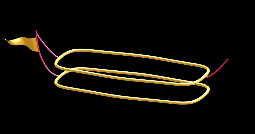
And, very last, we are going to add a flag attached to the outer cable. Let's make it flap in the wind. To make it we will recycle the z3 matrix again, but taper it based on its x-value. Then we will sinusoidally oscillate the flag in the y dimension as a function of x, constraining the y-position to be zero where it meets the cable. Lastly, we will displace it quadratically in the x-dimension as a function of z so that it lines up nicely with the rope. The phase of the sine-function is modified in the animation loop to give it a flapping motion.
h=linspace(0,1);
sc=10;
[fx,fz]=meshgrid(h,h-.5);
F=surf(sc*2.5*fx-90-2*(fz+.5).^2,sc*.3*erf(3*(1-h)).*sin(10*fx+n/5),sc*fz.*h+25,0*fx+c3,'Parent',P);
Plotting just the cables and flag shows:
Putting all the pieces together reveals the full airship:
A note about lighting: lighting and material properties really change the feel of the image you create. The above picture is rendered in a cartoony style by setting the specular exponent to a very low value (1), and adding lots of diffuse and ambient reflectivity as well. A light below the airship was also added, albeit with lower strength. Settings used for this plot were:
shading flat
view([0, 0]);
L=light;
L.Color = [1,1,1]/4;
light('position', [0, 0.5, 1], 'color', [1,1,1]);
light('position', [0, 1, -1], 'color', [1, 1, 1]/5);
material([1, 1, .7, 1])
set(gcf, 'color', 'k');
axis equal off
What about all the rest of the stuff (clouds, moon, atmospheric haze etc.) These were all (mostly) recycled bits from previous minihack entries. The clouds were made using power-law noise as explained in Adam Danz' blog post. The moon was borrowed from moonrun, but with an increased number of points. Atmospheric haze was recycled from Matlon5. The rest is just camera angles, hgtransform matrix updates, and updating alpha-maps or vertex coordinates.
Finally, the use of hann() adds the signal processing toolbox as a dependency. To avoid this use the following anonymous function:
hann = @(x)-cospi(linspace(0,2,x)')/2+.5;
I went to perform an IoT for an automated plantation but the same error always occurs to me when I upload it to the mcu node, which is: Connection to ThingSpeak failed.
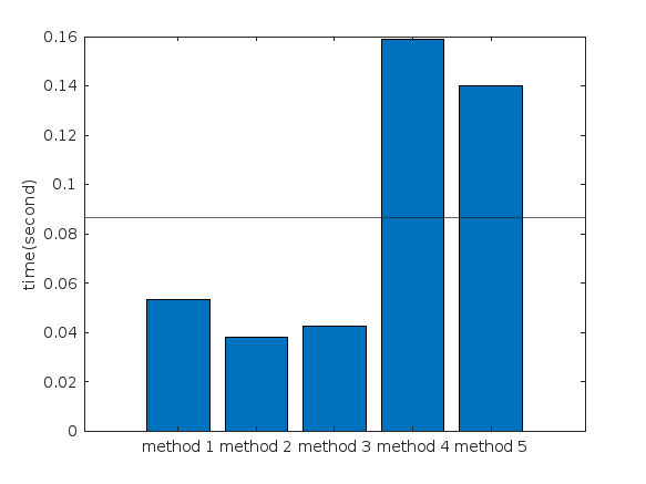
Create a struct arrays where each struct has field names "a," "b," and "c," which store different types of data. What efficient methods do you have to assign values from individual variables "a," "b," and "c" to each struct element? Here are five methods I've provided, listed in order of decreasing efficiency. What do you think?
Create an array of 10,000 structures, each containing each of the elements corresponding to the a,b,c variables.
num = 10000;
a = (1:num)';
b = string(a);
c = rand(3,3,num);
Here are the methods;
%% method1
t1 =tic;
s = struct("a",[], ...
"b",[], ...
"c",[]);
s1 = repmat(s,num,1);
for i = 1:num
s1(i).a = a(i);
s1(i).b = b(i);
s1(i).c = c(:,:,i);
end
t1 = toc(t1);
%% method2
t2 =tic;
for i = num:-1:1
s2(i).a = a(i);
s2(i).b = b(i);
s2(i).c = c(:,:,i);
end
t2 = toc(t2);
%% method3
t3 =tic;
for i = 1:num
s3(i).a = a(i);
s3(i).b = b(i);
s3(i).c = c(:,:,i);
end
t3 = toc(t3);
%% method4
t4 =tic;
ct = permute(c,[3,2,1]);
t = table(a,b,ct);
s4 = table2struct(t);
t4 = toc(t4);
%% method5
t5 =tic;
s5 = struct("a",num2cell(a),...
"b",num2cell(b),...
"c",squeeze(mat2cell(c,3,3,ones(num,1))));
t5 = toc(t5);
%% plot
bar([t1,t2,t3,t4,t5])
xtickformat('method %g')
ylabel("time(second)")
yline(mean([t1,t2,t3,t4,t5]))
Hot off the heels of my High Performance Computing experience in the Czech republic, I've just booked my flights to Atlanta for this year's supercomputing conference at SC24.
Will any of you be there?
syms u v
atan2alt(v,u)
function Z = atan2alt(V,U)
% extension of atan2(V,U) into the complex plane
Z = -1i*log((U+1i*V)./sqrt(U.^2+V.^2));
% check for purely real input. if so, zero out the imaginary part.
realInputs = (imag(U) == 0) & (imag(V) == 0);
Z(realInputs) = real(Z(realInputs));
end
As I am editing this post, I see the expected symbolic display in the nice form as have grown to love. However, when I save the post, it does not display. (In fact, it shows up here in the discussions post.) This seems to be a new problem, as I have not seen that failure mode in the past.
You can see the problem in this Answer forum response of mine, where it did fail.