メインコンテンツ
結果:
Well, this is my first time to participate in such community competitions and guess what, I've gone for 4 submissions so far (Feels Great!!)
So I wanna share some tricks that I followed for my first submission named Happy Shaping' ( Go Check it out!!):
1. Dynamic Background Color Change:
- Technique: The background color of the figure window is gradually changed using sine and cosine functions.
- Reason: These trigonometric functions (sin and cos) create smooth, oscillating transitions over time, which gives a fluid effect to the background's color shift.
- Implementation:
Color = [0.1 + 0.5*abs(sin(f/10)), 0.1 + 0.5*abs(cos(f/15)), 0.9 -
0.5*abs(sin(f/20))];
- Benefit: This introduces a smooth, visually appealing animation effect.
2. Smooth Object Motion Using Sine and Cosine:
- Technique: The position and shape of objects are based on trigonometric functions.
- Reason: Using sin(t) and cos(t) ensures that the movement is circular or elliptical, creating continuous and natural motion in animations.
- Implementation (for object position):
x = 10 * cos(t * 2 * pi) * (1 + 0.5 * sin(t * pi));
y = 10 * sin(t * 2 * pi) * (1 + 0.5 * cos(t * pi));
- Benefit: Circular and smooth motions are pleasing and easily controlled by tweaking the frequency and phase of sine/cosine functions.
3. Polygon Shape Changing Over Time:
- Technique: The number of sides of the polygon (sides) changes dynamically based on t.
- Reason: It creates variation in shape, maintaining user interest as the shape transitions from a triangle to a hexagon.
- Implementation:
sides = 3 + round(3 * abs(sin(t)));
- Benefit: This provides dynamic shape transitions over time, keeping the animation non-static.
4. Use of the fill Function for Color-Filled Shapes:
- Technique: The fill function is used to draw a polygon with smoothly changing colors.
- Reason: Filling polygons with varying colors based on time (t) allows for continuous color transitions, adding more complexity to the animation.
- Implementation:
fill(xp, yp, c, 'EdgeColor', 'none');
- Benefit: Combining both color changes and shape changes enhances the visual impact.
5. Consistent Use of hold on and hold off:
- Technique: hold on allows multiple graphic objects to be drawn on the same axes without clearing previous objects.
- Reason: This is crucial for drawing multiple elements (like polygons, circles, and lines) on the same figure.
- Benefit: It helps manage and layer different graphical elements effectively within the same frame.
6. Use of rectangle for a Smooth Ball Motion:
- Technique: The ball's motion is defined by rectangle with a Curvature of [1, 1] to make it circular.
- Reason: Using the rectangle function simplifies the process of drawing a filled circle, and controlling its position and size is intuitive.
- Benefit: It provides a straightforward way to animate circular objects within the plot.
7. Animating the Connection Line:
- Technique: A white dashed line (w--) is drawn between the polygon and the moving ball to show a connection between these objects.
- Reason: This adds interactivity to the scene, as it gives the impression that the polygon and the ball are related or connected in some way.
- Implementation:
plot([x bx], [y by], 'w--', 'LineWidth', 2);
- Benefit: A dynamic element that adds depth and narrative to the animation, guiding the viewer’s attention.
8. Frame Synchronization with Time (f and t):
- Technique: The variable f is used as a frame number, while t = f / 24 creates a link between frame and time.
- Reason: Ensuring smooth and continuous transitions in the animation over time is critical, so f acts as the control for time-based changes in shape, color, and position.
- Benefit: This makes it easy to manage frame rates and time-based updates for the animation.
Over the past week, we have seen many creative and compelling short movies! Now, let the voting begin! Cast your votes for the short movies you love. Authors, share your creations with friends, classmates, and colleagues. Let's showcase the beauty of mathematics to the world!
We know that one of the key goals for joining the Mini Hack contest is to LEARN! To celebrate knowledge sharing, we have special prizes—limited-edition MATLAB Shorts—up for grabs!

These exclusive prizes can only be earned through the MATLAB Shorts Mini Hack contest. Interested? Share your knowledge in the Discussions' general channel (be sure to add the tag 'contest2024') to earn opportunities to win the coveted MATLAB Shorts. You can share various types of content, such as tips and tricks for creating animations, background stories of your entry, or learnings you've gained from the contest. We will select different types of winners each week.

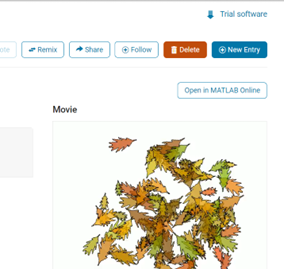
We also have an exciting feature announcement: you can now experiment with code in MATLAB Online. Simply click the 'Open in MATLAB Online' button above the movie preview section. Even better! ‘Open in MATLAB Online’ is also available in previous Mini Hack contests!

We look forward to seeing more amazing short movies in Week 2!
If you like them, please feel free to use them for free.
Try to install MATLAB2024a on Ubuntu24.04. In the image below, the button indicated by the green arrow is clickable, while the button indicated by the red arrow are unclickable, and input field where text cannot be entered, preventing the installation.

Do you use MATLAB Online for teaching? MATLAB Online lets students run MATLAB without having to install the software on the computer. All you need is a web browser and an internet connection.
I would love to hear comments and experiences of using MATLAB Online.
Let's say you have a chance to ask the MATLAB leadership team any question. What would you ask them?
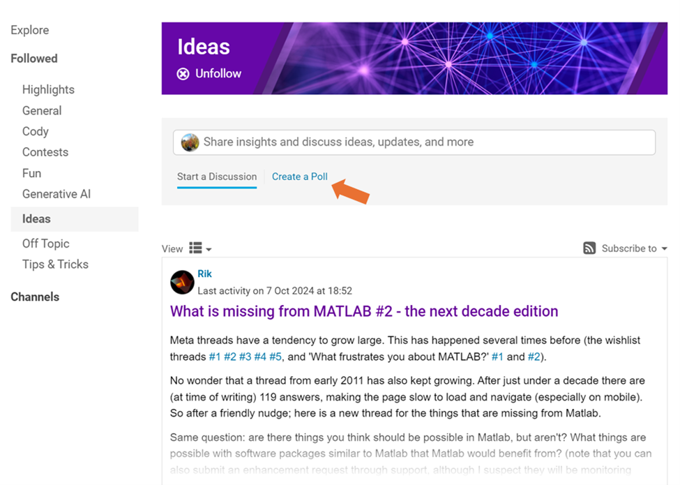
We are thrilled to announce that every community member now has the ability to create a poll in Discussions, allowing you to gather votes and opinions from the community.
How to create a poll:
You can find the ‘Create a Poll’ link just below the text box (see screenshot below). Please note that the default type of content is a ‘Discussion’. To start a poll, simply click the link.

Creating a poll is straightforward. You can add up to 6 choices for your poll and set the duration from 1 to 6 weeks.

Where to find the poll
Polls created by community members will appear only in the channel where they are created and the landing page of Discussions area. Discussions moderators have the privilege to feature/broadcast the poll across Answers, File Exchange, and Cody.
Thoughts?
We can’t wait to see what interesting polls our community will create. Meanwhile, if you have any questions or suggestions, feel free to leave a comment.
We're excited to announce that the 2024 Community Contest—MATLAB Shorts Mini Hack starts today! The contest will run for 5 weeks, from Oct. 7th to Nov. 10th.
What creative short movies will you create? Let the party begin, and we look forward to seeing you all in the contest!
If you are interested in AI, Autonomous Systems and Robotics, and the future of engineering, don't miss out on MATLAB EXPO 2024 and register now.
You will have the opportunity to connect with engineers, scientists, educators, and researchers, and new ideas.
Featured Sessions:
- From Embedded to Empowered: The Rise of Software-Defined Products - María Elena Gavilán Alfonso, MathWorks
- The Empathetic Engineers of Tomorrow - Dr. Darryll Pines, University of Maryland
- A Model-Based Design Journey from Aerospace to an Artificial Pancreas System - Louis Lintereur, Medtronic Diabetes
Featured Topics:
- AI
- Autonomous Systems and Robotics
- Electrification
- Algorithm Development and Data Analysis
- Modeling, Simulation, Verification, Validation, and Implementation
- Wireless Communications
- Cloud, Software Factories, and DevOps
- Preparing Future Engineers and Scientists

What is the side-effect of counting the number of Deep Learning Toolbox™ updates in the last 5 years? The industry has slowly stabilised and matured, so updates have slowed down in the last 1 year, and there has been no exponential growth.Is it correct to assume that? Let's see what you think!
releaseNumNames = "R"+string(2019:2024)+["a";"b"];
releaseNumNames = releaseNumNames(:);
numReleaseNotes = [10,14,27,39,38,43,53,52,55,57,46,46];
exampleNums = [nan,nan,nan,nan,nan,nan,40,24,22,31,24,38];
bar(releaseNumNames,[numReleaseNotes;exampleNums]')
legend(["#release notes","#new/update examples"],Location="northwest")
title("Number of Deep Learning Toolbox™ update items in the last 5 years")
ylabel("#release notes")
We are thrilled to announce the redesign of the Discussions leaf page, with a new user-focused right-hand column!

Why Are We Doing This?
- Address Readers’ Needs:
Previously, the right-hand column displayed related content, but feedback from our community indicated that this wasn't meeting your needs. Many of you expressed a desire to read more posts from the same author but found it challenging to locate them.
With the new design, readers can easily learn more about the author, explore their other posts, and follow them to receive notifications on new content.
- Enhance Authors’ Experience:
Since the launch of the Discussions area earlier this year, we've seen an influx of community members sharing insightful technical articles, use cases, and ideas. The new design aims to help you grow your followers and organize your content more effectively by editing tags. We highly encourage you to use the Discussions area as your community blogging platform.
We hope you enjoy the new design of the right-hand column. Please feel free to share your thoughts and experiences by leaving a comment below.
Dear contest participants,
The 2024 Community Contest—MATLAB Shorts Mini Hack—is just one week away! Last year, we challenged you to create a 48-frame, 2-second animation. This year, we're doubling the fun by increasing the frame count to 96 and adding audio support. Your mission? Create a short movie!
As always, whether you are a seasoned MATLAB user or just a beginner, you can participate in the contest and have opportunities to win amazing prizes.

Timeframe:
- The contest will run for 5 weeks, from Oct. 7th to Nov. 10th, Eastern Time.
General Rules:
- The first week is dedicated to entry creation, and the fifth week is reserved for voting only.
- Create a 96-frame, 4-second animation and add audio. We will loop it 3 times to create a 12-second short movie for you.
- The character limit remains at 2,000 characters.
Prizes
- You will have opportunities to win compelling prizes, including Amazon gift cards, MathWorks T-shirts, and virtual badges. We will give out both weekly prizes and grand prizes.
Warm-up!
With one week left before the contest begins, we recommend you warm up by reading a fantastic article: Walkthrough: making Little Nemo's airship in MATLAB by @Tim. The article shares both technical insights and the challenges encountered along the way.
The MATLAB Central Community Team
How can I mechanically couple synchronous reluctance motor from simscape electrical electromechanical library and dc generator from specialized power system library
We are excited to invite you to join our 2024 community contest – MATLAB Shorts Mini Hack! Last year, we challenged you to create a 48-frame animation. In 2024, we are increasing the frame count to 96 and supporting audio. Your mission? Create a short movie!
Whether you are a seasoned MATLAB user or just a beginner, you can participate in the contest and have opportunities to win amazing prizes. Be sure to check out our Blog post for more details on the Community Contests.
Timeframe
This contest runs for 5 weeks, from Oct. 7th to Nov. 10th.
How to Participate
- Create a new short movie or remix an existing one with up to 2,000 characters of code.
- Vote or comment on the short movies you love!
Prizes
You will have opportunities to win compelling prizes, including Amazon gift cards, MathWorks T-shirts, and virtual badges. We will give out both weekly prizes and grand prizes.
Stay Informed
Make sure to follow the contest to get important announcements and your prize updates.

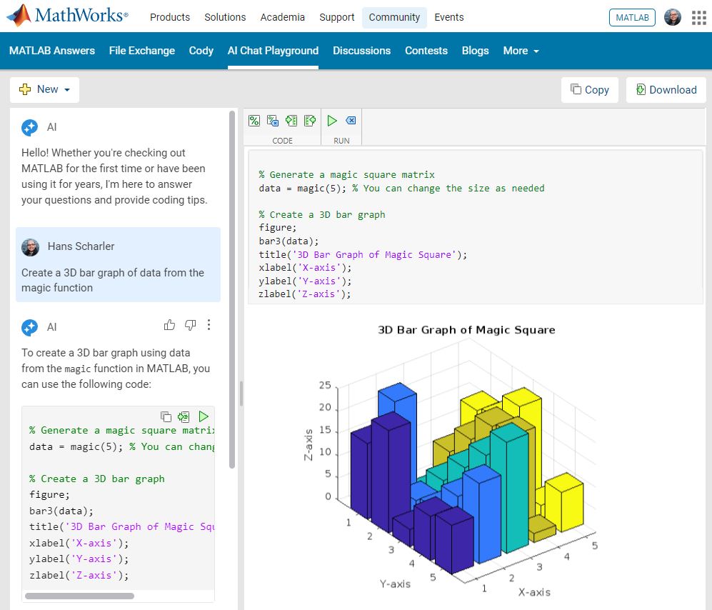
The AI Chat Playground at MATLAB Central has two new upgrades: OpenAI GPT-4o mini and MATLAB R2024b!
GPT-4o mini is a new language model from OpenAI and brings general knowledge up to October 2023. GPT-4o mini surpasses GPT-3.5 Turbo and other small models on academic benchmarks across both textual intelligence and reasoning. Our goal is to keep improving the output of the AI Chat Playground. This upgrade is available now: https://www.mathworks.com/matlabcentral/playground/
One more thing... we also updated the system to the latest release of MATLAB. This is R2024b and comes with hundreds of updates and new plot types to explore.Check out Mike Croucher's blog post about the latest version of MATLAB: https://blogs.mathworks.com/matlab/2024/09/13/the-latest-version-of-matlab-r2024b-has-just-been-released/
We are looking forward to your feedback on the updates to the AI Chat Playground. Let us know what you think and how you use this community app.

See the attached PDF for a higher resolution
Related blogs posts:
Always!
29%
It depends
14%
Never!
21%
I didn't know that was possible
36%
1810 票
Hello everyone,
Over the past few weeks, our community members have shared some incredible insights and resources. Here are some highlights worth checking out:
Interesting Questions
Johnathan is seeking help with implementing a complex equation into MATLAB's curve fitting toolbox. If you have experience with curve fitting or MATLAB, your input could be invaluable!
Popular Discussions
Athanasios continues his exploration of the Duffing Equation, delving into its chaotic behavior. It's a fascinating read for anyone interested in nonlinear dynamics or chaos theory.
John shares his playful exploration with MATLAB to find a generative equation for a sequence involving Fibonacci numbers. It's an intriguing challenge for those who love mathematical puzzles.
From File Exchange
Ayesha provides a graphical analysis of linearised models in epidemiology, offering a detailed look at the dynamics of these systems. This resource is perfect for those interested in mathematical modeling.
Gareth brings some humor to MATLAB with a toolbox designed to share jokes. It's a fun way to lighten the mood during conferences or meetups.
From the Blogs
Ned Gulley interviews Tim Marston, the 2023 MATLAB Mini Hack contest winner. Tim's creativity and skills are truly inspiring, and his story is a must-read for aspiring programmers.
Sivylla discusses the integration of AI with embedded systems, highlighting the benefits of using MATLAB and Simulink. It's an insightful read for anyone interested in the future of AI technology.
Thank you to all our contributors for sharing your knowledge and creativity. We encourage everyone to engage with these posts and continue fostering a vibrant and supportive community.
Happy exploring!
Explore the newest online training courses, available as of 2024b: one new Onramp, eight new short courses, and one new learning path. Yes, that’s 10 new offerings. We’ve been busy.
As a reminder, Onramps are free to all. Short courses and learning paths require a subscription to the Online Training Suite (OTS).
- Multibody Simulation Onramp
- Analyzing Results in Simulink
- Battery Pack Modeling
- Introduction to Motor Control
- Signal Processing Techniques for Streaming Signals
- Core Signal Processing Techniques in MATLAB (learning path – includes the four short courses listed below)
Hot off the heels of my High Performance Computing experience in the Czech republic, I've just booked my flights to Atlanta for this year's supercomputing conference at SC24.
Will any of you be there?


