結果:
For some time now, this has been bugging me - so I thought to gather some more feedback/information/opinions on this.
What would you classify Recursion? As a loop or as a vectorized section of code?
For context, this query occured to me while creating Cody problems involving strict (so to speak) vectorization - (Everyone is more than welcome to check my recent Cody questions).
To make problems interesting and/or difficult, I (and other posters) ban functions and functionalities - such as for loops, while loops, if-else statements, arrayfun() and the rest of the fun() family functions. However, some of the solutions including the reference solution I came up with for my latest problem, contained recursion.
I am rather divided on how to categorize it. What do you think?
Independent researcher: Nguyễn Khánh Tùng
ORCID: 0009-0002-9877-4137
Email: traiphieu.com@gmail.com
Website: https://traiphieu.com
Abstract
Every fundamental law of physics has a characteristic quantity and a unit of measurement (e.g., Newton for force, Joule for energy). The NKTg Law (Law of Varying Inertia) introduces a new physical quantity — varying inertia — defined by the interaction between position, velocity, and mass.
To measure this new quantity, I propose the NKTm unit, verified with NASA JPL Horizons data (Neptune, 2023–2024). Results indicate that NKTm is an independent fundamental unit, comparable in significance to Newton, Pascal, Joule, and Watt, with applications in astronomy, aerospace, and engineering.
This article clarifies the measurement unit of the NKTg Law (NKTm) and highlights its applications, many of which I have already implemented and shared as code examples on MATLAB Central.
1. Theoretical Basis
The NKTg Law describes motion under the combined effect of position (x), velocity (v), and mass (m):
NKTg=f(x,v,m)NKTg = f(x, v, m)NKTg=f(x,v,m)
Two expressions define varying inertia:
- NKTg₁ = x·p (Position–Momentum interaction)
- NKTg₂ = (dm/dt)·p (Mass-variation–Momentum interaction)
Both are measured by the same unit: NKTm.2. Dimensional Analysis
- From NKTg₁: [M⋅L2/T][M·L²/T][M⋅L2/T]
- From NKTg₂: [M2⋅L/T2][M²·L/T²][M2⋅L/T2]
Thus, NKTm is a unique unit that can take different dimensional forms depending on which component dominates.
For comparison:
QuantityUnitDimensionForceNewton (N)[M·L/T²]EnergyJoule (J)[M·L²/T²]PowerWatt (W)[M·L²/T³]Varying inertia (NKTg₁)NKTm[M·L²/T]Varying inertia (NKTg₂)NKTm[M²·L/T²]
3. Verification with NASA Data (Neptune, 2023–2024)
- Position (x): 4.498×1094.498 \times 10^94.498×10⁹ km
- Velocity (v): 5.43 km/s
- Mass (m): 1.0243×10261.0243 \times 10^{26}1.0243×1026 kg
- Momentum (p = m·v): 5.564×10265.564 \times 10^{26}5.564×1026 kg·m/s
Results:
- NKTg₁ = x·p ≈ 2.503 × 10³⁶ NKTm
- NKTg₂ ≈ -1.113 × 10²² NKTm (assumed micro gas escape)
- Total NKTg ≈ 2.501 × 10³⁶ NKTm
4. Applications
- Astronomy: describe planetary mass variation, star/galaxy formation, and long-term orbital stability.
- Aerospace: optimize rocket fuel usage, account for mass leakage, design ion/plasma engines.
- Earth sciences: analyze GRACE-FO data, model ice melting, sea-level rise, and mass redistribution.
- Engineering: variable-mass robotics, cargo systems, vibration analysis, fluid/particle simulations.
👉 Many of these applications are already available as MATLAB code examples that I have uploaded to MATLAB Central, showing how NKTm can be computed and applied in practice.5. Scientific Significance
- Establishes a new fundamental unit (NKTm), independent of Newton and Joule.
- Provides a theoretical framework for variable-mass dynamics, beyond Newton and Einstein.
- Supports accurate computation and simulation of real-world systems with mass variation.
Conclusion
The introduction of the NKTm unit demonstrates that varying inertia is a measurable, independent physical quantity. Like Newton or Joule, NKTm lays the foundation for a new reference system in physics, with applications ranging from planetary mechanics to modern space technology.
This article not only clarifies the measurement standard of the NKTg Law, but also connects directly with practical MATLAB implementations for simulation and verification.
Discussion prompt:
What do you think about introducing a new physical unit like NKTm? Could it be integrated into MATLAB-based simulation frameworks for variable-mass systems?
You can refer to the following four related articles to gain a deeper understanding of the NKTg Law and its applications
I came across this fun video from @Christoper Lum, and I have to admit—his MathWorks swag collection is pretty impressive! He’s got pieces I even don’t have.
So now I’m curious… what MathWorks swag do you have hiding in your office or closet?
- Which one is your favorite?
- Which ones do you want to add to your collection?
Show off your swag and share it with the community! 🚀
Since R2024b, a Levenberg–Marquardt solver (TrainingOptionsLM) was introduced. The built‑in function trainnet now accepts training options via the trainingOptions function (https://www.mathworks.com/help/deeplearning/ref/trainingoptions.html#bu59f0q-2) and supports the LM algorithm. I have been curious how to use it in deep learning, and the official documentation has not provided a concrete usage example so far. Below I give a simple example to illustrate how to use this LM algorithm to optimize a small number of learnable parameters.
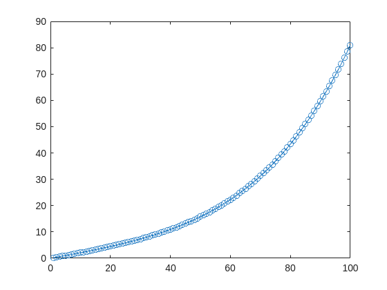
For example, consider the nonlinear function:
y_hat = @(a,t) a(1)*(t/100) + a(2)*(t/100).^2 + a(3)*(t/100).^3 + a(4)*(t/100).^4;
It represents a curve. Given 100 matching points (t → y_hat), we want to use least squares to estimate the four parameters a1–a4.
t = (1:100)';
y_hat = @(a,t)a(1)*(t/100) + a(2)*(t/100).^2 + a(3)*(t/100).^3 + a(4)*(t/100).^4;
x_true = [ 20 ; 10 ; 1 ; 50 ];
y_true = y_hat(x_true,t);
plot(t,y_true,'o-')
- Using the traditional lsqcurvefit-wrapped "Levenberg–Marquardt" algorithm:
x_guess = [ 5 ; 2 ; 0.2 ; -10 ];
options = optimoptions("lsqcurvefit",Algorithm="levenberg-marquardt",MaxFunctionEvaluations=800);
[x,resnorm,residual,exitflag] = lsqcurvefit(y_hat,x_guess,t,y_true,-50*ones(4,1),60*ones(4,1),options);
x,resnorm,exitflag
- Using the deep-learning-wrapped "Levenberg–Marquardt" algorithm:
options = trainingOptions("lm", ...
InitialDampingFactor=0.002, ...
MaxDampingFactor=1e9, ...
DampingIncreaseFactor=12, ...
DampingDecreaseFactor=0.2,...
GradientTolerance=1e-6, ...
StepTolerance=1e-6,...
Plots="training-progress");
numFeatures = 1;
layers = [featureInputLayer(numFeatures,'Name','input')
fitCurveLayer(Name='fitCurve')];
net = dlnetwork(layers);
XData = dlarray(t);
YData = dlarray(y_true);
netTrained = trainnet(XData,YData,net,"mse",options);
netTrained.Layers(2)
classdef fitCurveLayer < nnet.layer.Layer ...
& nnet.layer.Acceleratable
% Example custom SReLU layer.
properties (Learnable)
% Layer learnable parameters
a1
a2
a3
a4
end
methods
function layer = fitCurveLayer(args)
arguments
args.Name = "lm_fit";
end
% Set layer name.
layer.Name = args.Name;
% Set layer description.
layer.Description = "fit curve layer";
end
function layer = initialize(layer,~)
% layer = initialize(layer,layout) initializes the layer
% learnable parameters using the specified input layout.
if isempty(layer.a1)
layer.a1 = rand();
end
if isempty(layer.a2)
layer.a2 = rand();
end
if isempty(layer.a3)
layer.a3 = rand();
end
if isempty(layer.a4)
layer.a4 = rand();
end
end
function Y = predict(layer, X)
% Y = predict(layer, X) forwards the input data X through the
% layer and outputs the result Y.
% Y = layer.a1.*exp(-X./layer.a2) + layer.a3.*X.*exp(-X./layer.a4);
Y = layer.a1*(X/100) + layer.a2*(X/100).^2 + layer.a3*(X/100).^3 + layer.a4*(X/100).^4;
end
end
end
The network is very simple — only the fitCurveLayer defines the learnable parameters a1–a4. I observed that the output values are very close to those from lsqcurvefit.

trainingOptions - Options for training deep learning neural network - MATLAB
This MATLAB function returns training options for the optimizer specified by solverName.
I saw this YouTube short on my feed: What is MATLab?

I was mostly mesmerized by the minecraft gameplay going on in the background.
Found it funny, thought i'd share.
Trinity
- It's the question that drives us, Neo. It's the question that brought you here. You know the question, just as I did.
Neo
- What is the Matlab?
Morpheus
- Unfortunately, no one can be told what the Matlab is. You have to see it for yourself.
And also later :
Morpheus
- The Matlab is everywhere. It is all around us. Even now, in this very room. You can feel it when you go to work [...]
The Architect
- The first Matlab I designed was quite naturally perfect. It was a work of art. Flawless. Sublime.
[My Matlab quotes version of the movie (Matrix, 1999) ]
Function Syntax Design Conundrum
As a MATLAB enthusiast, I particularly enjoy Steve Eddins' blog and the cool things he explores. MATLAB's new argument blocks are great, but there's one frustrating limitation that Steve outlined beautifully in his blog post "Function Syntax Design Conundrum": cases where an argument should accept both enumerated values AND other data types.
Steve points out this could be done using the input parser, but I prefer having tab completions and I'm not a fan of maintaining function signature JSON files for all my functions.
Personal Context on Enumerations
To be clear: I honestly don't like enumerations in any way, shape, or form. One reason is how awkward they are. I've long suspected they're simply predefined constructor calls with a set argument, and I think that's all but confirmed here. This explains why I've had to fight the enumeration system when trying to take arguments of many types and normalize them to enumerated members, or have numeric values displayed as enumerated members without being recast to the superclass every operation.
The Discovery
While playing around extensively with metadata for another project, I realized (and I'm entirely unsure why it took so long) that the properties of a metaclass object are just, in many cases, the attributes of the classdef. In this realization, I found a solution to Steve's and my problem.
To be clear: I'm not in love with this solution. I would much prefer a better approach for allowing variable sets of membership validation for arguments. But as it stands, we don't have that, so here's an interesting, if incredibly hacky, solution.
If you call struct() on a metaclass object to view its hidden properties, you'll notice that in addition to the public "Enumeration" property, there's a hidden "Enumerable" property. They're both logicals, which implies they're likely functionally distinct. I was curious about that distinction and hoped to find some functionality by intentionally manipulating these values - and I did, solving the exact problem Steve mentions.
The Problem Statement
We have a function with an argument that should allow "dual" input types: enumerated values (Steve's example uses days of the week, mine uses the "all" option available in various dimension-operating functions) AND integers. We want tab completion for the enumerated values while still accepting the numeric inputs.
A Solution for Tab-Completion Supported Arguments
Rather than spoil Steve's blog post, let me use my own example: implementing a none() function. The definition is simple enough tf = ~any(A, dim); but when we wrap this in another function, we lose the tab-completion that any() provides for the dim argument (which gives you "all"). There's no great way to implement this as a function author currently - at least, that's well documented.
So here's my solution:
%% Example Function Implementation
% This is a simple implementation of the DimensionArgument class for implementing dual type inputs that allow enumerated tab-completion.
function tf = none(A, dim)
arguments(Input)
A logical;
dim DimensionArgument = DimensionArgument(A, true);
end
% Simple example (notice the use of uplus to unwrap the hidden property)
tf = ~any(A, +dim);
end
I like this approach because the additional work required to implement it, once the enumeration class is initialized, is minimal. Here are examples of function calls, note that the behavior parallels that of the MATLAB native-style tab-completion:
%% Test Data
% Simple logical array for testing
A = randi([0, 1], [3, 5], "logical");
%% Example function calls
tf = none(A, "all"); % This is the tab-completion it's 1:1 with MATLABs behavior
tf = none(A, [1, 2]); % We can still use valid arguments (validated in the constructor)
tf = none(A); % Showcase of the constructors use as a default argument generator
How It Works
What makes this work is the previously mentioned Enumeration attribute. By setting Enumeration = false while still declaring an enumeration block in the classdef file, we get the suggested members as auto-complete suggestions. As I hinted at, the value of enumerations (if you don't subclass a builtin and define values with the someMember (1) syntax) are simply arguments to constructor calls.
We also get full control over the storage and handling of the class, which means we lose the implicit storage that enumerations normally provide and are responsible for doing so ourselves - but I much prefer this. We can implement internal validation logic to ensure values that aren't in the enumerated set still comply with our constraints, and store the input (whether the enumerated member or alternative type) in an internal property.
As seen in the example class below, this maintains a convenient interface for both the function caller and author the only particuarly verbose portion is the conversion methods... Which if your willing to double down on the uplus unwrapping context can be avoided. What I have personally done is overload the uplus function to return the input (or perform the identity property) this allowss for the uplus to be used universally to unwrap inputs and for those that cant, and dont have a uplus definition, the value itself is just returned:
classdef(Enumeration = false) DimensionArgument % < matlab.mixin.internal.MatrixDisplay
%DimensionArgument Enumeration class to provide auto-complete on functions needing the dimension type seen in all()
% Enumerations are just macros to make constructor calls with a known set of arguments. Declaring the 'all'
% enumeration member means this class can be set as the type for an input and the auto-completion for the given
% argument will show the enumeration members, allowing tab-completion. Declaring the Enumeration attribute of
% the class as false gives us control over the constructor and internal implementation. As such we can use it
% to validate the numeric inputs, in the event the 'all' option was not used, and return an object that will
% then work in place of valid dimension argument options.
%% Enumeration members
% These are the auto-complete options you'd like to make available for the function signature for a given
% argument.
enumeration(Description="Enumerated value for the dimension argument.")
all
end
%% Properties
% The internal property allows the constructor's input to be stored; this ensures that the value is store and
% that the output of the constructor has the class type so that the validation passes.
% (Constructors must return the an object of the class they're a constructor for)
properties(Hidden, Description="Storage of the constructor input for later use.")
Data = [];
end
%% Constructor method
% By the magic of declaring (Enumeration = false) in our class def arguments we get full control over the
% constructor implementation.
%
% The second argument in this specific instance is to enable the argument's default value to be set in the
% arguments block itself as opposed to doing so in the function body... I like this better but if you didn't
% you could just as easily keep the constructor simple.
methods
function obj = DimensionArgument(A, Adim)
%DimensionArgument Initialize the dimension argument.
arguments
% This will be the enumeration member name from auto-completed entries, or the raw user input if not
% used.
A = [];
% A flag that indicates to create the value using different logic, in this case the first non-singleton
% dimension, because this matches the behavior of functions like, all(), sum() prod(), etc.
Adim (1, 1) logical = false;
end
if(Adim)
% Allows default initialization from an input to match the aforemention function's behavior
obj.Data = firstNonscalarDim(A);
else
% As a convenience for this style of implementation we can validate the input to ensure that since we're
% suppose to be an enumeration, the input is valid
DimensionArgument.mustBeValidMember(A);
% Store the input in a hidden property since declaring ~Enumeration means we are responsible for storing
% it.
obj.Data = A;
end
end
end
%% Conversion methods
% Applies conversion to the data property so that implicit casting of functions works. Unfortunately most of
% the MathWorks defined functions use a different system than that employed by the arguments block, which
% defers to the class defined converter methods... Which is why uplus (+obj) has been defined to unwrap the
% data for ease of use.
methods
function obj = uplus(obj)
obj = obj.Data;
end
function str = char(obj)
str = char(obj.Data);
end
function str = cellstr(obj)
str = cellstr(obj.Data);
end
function str = string(obj)
str = string(obj.Data);
end
function A = double(obj)
A = double(obj.Data);
end
function A = int8(obj)
A = int8(obj.Data);
end
function A = int16(obj)
A = int16(obj.Data);
end
function A = int32(obj)
A = int32(obj.Data);
end
function A = int64(obj)
A = int64(obj.Data);
end
end
%% Validation methods
% These utility methods are for input validation
methods(Static, Access = private)
function tf = isValidMember(obj)
%isValidMember Checks that the input is a valid dimension argument.
tf = (istext(obj) && all(obj == "all", "all")) || (isnumeric(obj) && all(isint(obj) & obj > 0, "all"));
end
function mustBeValidMember(obj)
%mustBeValidMember Validates that the input is a valid dimension argument for the dim/dimVec arguments.
if(~DimensionArgument.isValidMember(obj))
exception("JB:DimensionArgument:InvalidInput", "Input must be an integer value or the term 'all'.")
end
end
end
%% Convenient data display passthrough
methods
function disp(obj, name)
arguments
obj DimensionArgument
name string {mustBeScalarOrEmpty} = [];
end
% Dispatch internal data's display implementation
display(obj.Data, char(name));
end
end
end
In the event you'd actually play with theres here are the function definitions for some of the utility functions I used in them, including my exception would be a pain so i wont, these cases wont use it any...
% Far from my definition isint() but is consistent with mustBeInteger() for real numbers but will suffice for the example
function tf = isint(A)
arguments
A {mustBeNumeric(A)};
end
tf = floor(A) == A
end
% Sort of the same but its fine
function dim = firstNonscalarDim(A)
arguments
A
end
dim = [find(size(A) > 1, 1), 0];
dim(1) = dim(1);
end
Hello MATLAB Central, this is my first article.
My name is Yann. And I love MATLAB.
I also love HTTP (i know, weird fetish)
So i started a conversation with ChatGPT about it:
gitclone('https://github.com/yanndebray/HTTP-with-MATLAB');
cd('HTTP-with-MATLAB')
http_with_MATLAB
I'm not sure that this platform is intended to clone repos from github, but i figured I'd paste this shortcut in case you want to try out my live script http_with_MATLAB.m
A lot of what i program lately relies on external web services (either for fetching data, or calling LLMs).
So I wrote a small tutorial of the 7 or so things I feel like I need to remember when making HTTP requests in MATLAB.
Let me know what you think
Did you know that function double with string vector input significantly outperforms str2double with the same input:
x = rand(1,50000);
t = string(x);
tic; str2double(t); toc
tic; I1 = str2double(t); toc
tic; I2 = double(t); toc
isequal(I1,I2)
Recently I needed to parse numbers from text. I automatically tried to use str2double. However, profiling revealed that str2double was the main bottleneck in my code. Than I realized that there is a new note (since R2024a) in the documentation of str2double:
"Calling string and then double is recommended over str2double because it provides greater flexibility and allows vectorization. For additional information, see Alternative Functionality."
Independent researcher: Nguyễn Khánh Tùng
ORCID: 0009-0002-9877-4137
Email: traiphieu.com@gmail.com
Website: https://traiphieu.com
The NKTg Law (Law of Variable Inertia) not only holds value in physics but also opens up wide possibilities for applications in programming and simulation. The remarkable point here is that the same law, the same formula, can be implemented across a wide range of different programming languages.
In the content below, you will find a collection of 30 code snippets, each corresponding to one of the world’s leading programming languages:
Python, C++, Java, C, C#, JavaScript, SQL, Go (Golang), PHP, TypeScript, Swift, Kotlin, Rust, Ruby, R, MATLAB, Perl, Dart, Scala, Visual Basic, Assembly, Shell (Bash), Objective-C, Haskell, Lua, Ada, Groovy, Delphi/Object Pascal, COBOL, and Fortran.
All the code snippets illustrate how to calculate the fundamental quantities of The NKTg Law on Varying Inertia:
The movement tendency of an object in space depends on the relationship between its position, velocity, and mass.
NKTg = f(x, v, m)
In which:
- x is the position or displacement of the object relative to the reference point.
- v is the velocity.
- m is the mass.
The movement tendency of the object is determined by the following basic product quantities:
NKTg₁ = x × p
NKTg₂ = (dm/dt) × p
In which:
- p is the linear momentum, calculated by p = m × v.
- dm/dt is the rate of mass change over time.
- NKTg₁ is the quantity representing the product of position and momentum.
- NKTg₂ is the quantity representing the product of mass variation and momentum.
- The unit of measurement is NKTm, representing a unit of varying inertia.
The sign and value of the two quantities NKTg₁ and NKTg₂ determine the movement tendency:
- If NKTg₁ is positive, the object tends to move away from the stable state.
- If NKTg₁ is negative, the object tends to move toward the stable state.
- If NKTg₂ is positive, the mass variation has a supporting effect on the movement.
- If NKTg₂ is negative, the mass variation has a resisting effect on the movement.
The stable state in this law is understood as the state in which the position (x), velocity (v), and mass (m) of the object interact with each other to maintain the movement structure, helping the object avoid losing control and preserving its inherent movement pattern.
Implementing the same law across 30 programming ecosystems demonstrates its universality and flexibility, while also confirming that any language—whether general-purpose and popular, or specialized and classical—can apply the NKTg Law to simulate, analyze, and handle practical problems.
You can refer to the following four related articles to gain a deeper understanding of the NKTg Law and its applications
作ったコードは公開して使ってもらいましょう!ということでその方法をブログで紹介します。
GitHub や File Exchange で公開しているコードがあれば、ぜひこのスレで教えてください!
ブログで紹介している大まかな3ステップをここにまとめます。
1. GitHub でコードを公開・開発する
- GitHub 上でのリポジトリ公開はコミュニティ形成にもつながります。
- R2025a 以降は MATLAB の Markdown サポートも強化されており、README.md を充実させると理解や導入が促進されます。
2. File Exchange に展開(GitHub と連携して自動同期)
- File Exchangeで公開することで MATLAB 内から検索・インストールが可能になります。
- GitHub と File Exchange の連携設定により、GitHub の更新を自動的に File Exchange に反映させることも可能です。
3. 「Open in MATLAB Online」ボタンやリンクを追加
- GitHub リポジトリに「Open in MATLAB Online」リンクやボタンを埋め込むことで、ブラウザ上でコードを試せます。
Hey cody fellows :-) !
I recently created two problem groups, but as you can see I struggle to set their cover images :
What is weird given :
- I already did it successfully twice in the past for my previous groups ;
- If you take one problem specifically, Problem 60984. Mesh the icosahedron for instance, you can normally see the icon of the cover image in the top right hand corner, can't you ?
- I always manage to set cover images to my contributions (mostly in the filexchange).
I already tried several image formats, included .png 4/3 ratio, but still the cover images don't set.
Could you please help me to correctly set my cover images ?
Thank you.
Nicolas
Resharing a fun short video explaining what MATLAB is. :)
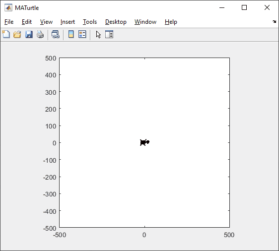
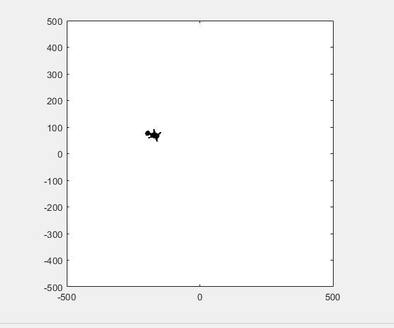
t = turtle(); % Start a turtle
t.forward(100); % Move forward by 100
t.backward(100); % Move backward by 100
t.left(90); % Turn left by 90 degrees
t.right(90); % Tur right by 90 degrees
t.goto(100, 100); % Move to (100, 100)
t.turnto(90); % Turn to 90 degrees, i.e. north
t.speed(1000); % Set turtle speed as 1000 (default: 500)
t.pen_up(); % Pen up. Turtle leaves no trace.
t.pen_down(); % Pen down. Turtle leaves a trace again.
t.color('b'); % Change line color to 'b'
t.begin_fill(FaceColor, EdgeColor, FaceAlpha); % Start filling
t.end_fill(); % End filling
t.change_icon('person.png'); % Change the icon to 'person.png'
t.clear(); % Clear the Axes
classdef turtle < handle
properties (GetAccess = public, SetAccess = private)
x = 0
y = 0
q = 0
end
properties (SetAccess = public)
speed (1, 1) double = 500
end
properties (GetAccess = private)
speed_reg = 100
n_steps = 20
ax
l
ht
im
is_pen_up = false
is_filling = false
fill_color
fill_alpha
end
methods
function obj = turtle()
figure(Name='MATurtle', NumberTitle='off')
obj.ax = axes(box="on");
hold on,
obj.ht = hgtransform();
icon = flipud(imread('turtle.png'));
obj.im = imagesc(obj.ht, icon, ...
XData=[-30, 30], YData=[-30, 30], ...
AlphaData=(255 - double(rgb2gray(icon)))/255);
obj.l = plot(obj.x, obj.y, 'k');
obj.ax.XLim = [-500, 500];
obj.ax.YLim = [-500, 500];
obj.ax.DataAspectRatio = [1, 1, 1];
obj.ax.Toolbar.Visible = 'off';
disableDefaultInteractivity(obj.ax);
end
function home(obj)
obj.x = 0;
obj.y = 0;
obj.ht.Matrix = eye(4);
end
function forward(obj, dist)
obj.step(dist);
end
function backward(obj, dist)
obj.step(-dist)
end
function step(obj, delta)
if numel(delta) == 1
delta = delta*[cosd(obj.q), sind(obj.q)];
end
if obj.is_filling
obj.fill(delta);
else
obj.move(delta);
end
end
function goto(obj, x, y)
dx = x - obj.x;
dy = y - obj.y;
obj.turnto(rad2deg(atan2(dy, dx)));
obj.step([dx, dy]);
end
function left(obj, q)
obj.turn(q);
end
function right(obj, q)
obj.turn(-q);
end
function turnto(obj, q)
obj.turn(obj.wrap_angle(q - obj.q, -180));
end
function pen_up(obj)
if obj.is_filling
warning('not available while filling')
return
end
obj.is_pen_up = true;
end
function pen_down(obj, go)
if obj.is_pen_up
if nargin == 1
obj.l(end+1) = plot(obj.x, obj.y, Color=obj.l(end).Color);
else
obj.l(end+1) = go;
end
uistack(obj.ht, 'top')
end
obj.is_pen_up = false;
end
function color(obj, line_color)
if obj.is_filling
warning('not available while filling')
return
end
obj.pen_up();
obj.pen_down(plot(obj.x, obj.y, Color=line_color));
end
function begin_fill(obj, FaceColor, EdgeColor, FaceAlpha)
arguments
obj
FaceColor = [.6, .9, .6];
EdgeColor = [0 0.4470 0.7410];
FaceAlpha = 1;
end
if obj.is_filling
warning('already filling')
return
end
obj.fill_color = FaceColor;
obj.fill_alpha = FaceAlpha;
obj.pen_up();
obj.pen_down(patch(obj.x, obj.y, [1, 1, 1], ...
EdgeColor=EdgeColor, FaceAlpha=0));
obj.is_filling = true;
end
function end_fill(obj)
if ~obj.is_filling
warning('not filling now')
return
end
obj.l(end).FaceColor = obj.fill_color;
obj.l(end).FaceAlpha = obj.fill_alpha;
obj.is_filling = false;
end
function change_icon(obj, filename)
icon = flipud(imread(filename));
obj.im.CData = icon;
obj.im.AlphaData = (255 - double(rgb2gray(icon)))/255;
end
function clear(obj)
obj.x = 0;
obj.y = 0;
delete(obj.ax.Children(2:end));
obj.l = plot(0, 0, 'k');
obj.ht.Matrix = eye(4);
end
end
methods (Access = private)
function animated_step(obj, delta, q, initFcn, updateFcn)
arguments
obj
delta
q
initFcn = @() []
updateFcn = @(~, ~) []
end
dx = delta(1)/obj.n_steps;
dy = delta(2)/obj.n_steps;
dq = q/obj.n_steps;
pause_duration = norm(delta)/obj.speed/obj.speed_reg;
initFcn();
for i = 1:obj.n_steps
updateFcn(dx, dy);
obj.ht.Matrix = makehgtform(...
translate=[obj.x + dx*i, obj.y + dy*i, 0], ...
zrotate=deg2rad(obj.q + dq*i));
pause(pause_duration)
drawnow limitrate
end
obj.x = obj.x + delta(1);
obj.y = obj.y + delta(2);
end
function obj = turn(obj, q)
obj.animated_step([0, 0], q);
obj.q = obj.wrap_angle(obj.q + q, 0);
end
function move(obj, delta)
initFcn = @() [];
updateFcn = @(dx, dy) [];
if ~obj.is_pen_up
initFcn = @() initializeLine();
updateFcn = @(dx, dy) obj.update_end_point(obj.l(end), dx, dy);
end
function initializeLine()
obj.l(end).XData(end+1) = obj.l(end).XData(end);
obj.l(end).YData(end+1) = obj.l(end).YData(end);
end
obj.animated_step(delta, 0, initFcn, updateFcn);
end
function obj = fill(obj, delta)
initFcn = @() initializePatch();
updateFcn = @(dx, dy) obj.update_end_point(obj.l(end), dx, dy);
function initializePatch()
obj.l(end).Vertices(end+1, :) = obj.l(end).Vertices(end, :);
obj.l(end).Faces = 1:size(obj.l(end).Vertices, 1);
end
obj.animated_step(delta, 0, initFcn, updateFcn);
end
end
methods (Static, Access = private)
function update_end_point(l, dx, dy)
l.XData(end) = l.XData(end) + dx;
l.YData(end) = l.YData(end) + dy;
end
function q = wrap_angle(q, min_angle)
q = mod(q - min_angle, 360) + min_angle;
end
end
end
I would like to zoom directly on the selected region when using  on my image created with image or imagesc. First of all, I would recommend using image or imagesc and not imshow for this case, see comparison here: Differences between imshow() and image()? However when zooming Stretch-to-Fill behavior happens and I don't want that. Try range zoom to image generated by this code:
fig = uifigure;
ax = uiaxes(fig);
im = imread("peppers.png");
h = imagesc(im,"Parent",ax);
axis(ax,'tight', 'off')
I can fix that with manualy setting data aspect ratio:
daspect(ax,[1 1 1])
However, I need this code to run automatically after zooming. So I create zoom object and ActionPostCallback which is called everytime after I zoom, see zoom - ActionPostCallback.
z = zoom(ax);
z.ActionPostCallback = @(fig,ax) daspect(ax.Axes,[1 1 1]);
If you need, you can also create ActionPreCallback which is called everytime before I zoom, see zoom - ActionPreCallback.
z.ActionPreCallback = @(fig,ax) daspect(ax.Axes,'auto');
Code written and run in R2025a.
I am thrilled python interoperability now seems to work for me with my APPLE M1 MacBookPro and MATLAB V2025a. The available instructions are still, shall we say, cryptic. Here is a summary of my interaction with GPT 4o to get this to work.
===========================================================
MATLAB R2025a + Python (Astropy) Integration on Apple Silicon (M1/M2/M3 Macs)
===========================================================
Author: D. Carlsmith, documented with ChatGPT
Last updated: July 2025
This guide provides full instructions, gotchas, and workarounds to run Python 3.10 with MATLAB R2025a (Apple Silicon/macOS) using native ARM64 Python and calling modules like Astropy, Numpy, etc. from within MATLAB.
===========================================================
Overview
===========================================================
- MATLAB R2025a on Apple Silicon (M1/M2/M3) runs as "maca64" (native ARM64).
- To call Python from MATLAB, the Python interpreter must match that architecture (ARM64).
- Using Intel Python (x86_64) with native MATLAB WILL NOT WORK.
- The cleanest solution: use Miniforge3 (Conda-forge's lightweight ARM64 distribution).
===========================================================
1. Install Miniforge3 (ARM64-native Conda)
===========================================================
In Terminal, run:
curl -LO https://github.com/conda-forge/miniforge/releases/latest/download/Miniforge3-MacOSX-arm64.sh
bash Miniforge3-MacOSX-arm64.sh
Follow prompts:
- Press ENTER to scroll through license.
- Type "yes" when asked to accept the license.
- Press ENTER to accept the default install location: ~/miniforge3
- When asked:
Do you wish to update your shell profile to automatically initialize conda? [yes|no]
Type: yes
===========================================================
2. Restart Terminal and Create a Python Environment for MATLAB
===========================================================
Run the following:
conda create -n matlab python=3.10 astropy numpy -y
conda activate matlab
Verify the Python path:
which python
Expected output:
/Users/YOURNAME/miniforge3/envs/matlab/bin/python
===========================================================
3. Verify Python + Astropy From Terminal
===========================================================
Run:
python -c "import astropy; print(astropy.__version__)"
Expected output:
6.x.x (or similar)
===========================================================
4. Configure MATLAB to Use This Python
===========================================================
In MATLAB R2025a (Apple Silicon):
clear classes
pyenv('Version', '/Users/YOURNAME/miniforge3/envs/matlab/bin/python')
py.sys.version
You should see the Python version printed (e.g. 3.10.18). No error means it's working.
===========================================================
5. Gotchas and Their Solutions
===========================================================
❌ Error: Python API functions are not available
→ Cause: Wrong architecture or broken .dylib
→ Fix: Use Miniforge ARM64 Python. DO NOT use Intel Anaconda.
❌ Error: Invalid text character (↑ points at __version__)
→ Cause: MATLAB can’t parse double underscores typed or pasted
→ Fix: Use: py.getattr(module, '__version__')
❌ Error: Unrecognized method 'separation' or 'sec'
→ Cause: MATLAB can't reflect dynamic Python methods
→ Fix: Use: py.getattr(obj, 'method')(args)
===========================================================
6. Run Full Verification in MATLAB
===========================================================
Paste this into MATLAB:
% Set environment
clear classes
pyenv('Version', '/Users/YOURNAME/miniforge3/envs/matlab/bin/python');
% Import modules
coords = py.importlib.import_module('astropy.coordinates');
time_mod = py.importlib.import_module('astropy.time');
table_mod = py.importlib.import_module('astropy.table');
% Astropy version
ver = char(py.getattr(py.importlib.import_module('astropy'), '__version__'));
disp(['Astropy version: ', ver]);
% SkyCoord angular separation
c1 = coords.SkyCoord('10h21m00s', '+41d12m00s', pyargs('frame', 'icrs'));
c2 = coords.SkyCoord('10h22m00s', '+41d15m00s', pyargs('frame', 'icrs'));
sep_fn = py.getattr(c1, 'separation');
sep = sep_fn(c2);
arcsec = double(sep.to('arcsec').value);
fprintf('Angular separation = %.3f arcsec\n', arcsec);
% Time difference in seconds
Time = time_mod.Time;
t1 = Time('2025-01-01T00:00:00', pyargs('format','isot','scale','utc'));
t2 = Time('2025-01-02T00:00:00', pyargs('format','isot','scale','utc'));
dt = py.getattr(t2, '__sub__')(t1);
seconds = double(py.getattr(dt, 'sec'));
fprintf('Time difference = %.0f seconds\n', seconds);
% Astropy table display
tbl = table_mod.Table(pyargs('names', {'a','b'}, 'dtype', {'int','float'}));
tbl.add_row({1, 2.5});
tbl.add_row({2, 3.7});
disp(tbl);
===========================================================
7. Optional: Automatically Configure Python in startup.m
===========================================================
To avoid calling pyenv() every time, edit your MATLAB startup:
edit startup.m
Add:
try
pyenv('Version', '/Users/YOURNAME/miniforge3/envs/matlab/bin/python');
catch
warning("Python already loaded.");
end
===========================================================
8. Final Notes
===========================================================
- This setup avoids all architecture mismatches.
- It uses a clean, minimal ARM64 Python that integrates seamlessly with MATLAB.
- Do not mix Anaconda (Intel) with Apple Silicon MATLAB.
- Use py.getattr for any Python attribute containing underscores or that MATLAB can't resolve.
You can now run NumPy, Astropy, Pandas, Astroquery, Matplotlib, and more directly from MATLAB.
===========================================================
群馬産業技術センター様をお招きし、製造現場での異常検知の取り組みについてご紹介いただくオンラインセミナーを開催します。
実際の開発事例を通して、MATLABを使った「教師なし」異常検知の進め方や、予知保全に役立つ最新機能もご紹介します。
✅ 異常検知・予知保全に興味がある方
✅ データ活用を何から始めればいいか迷っている方
✅ 実際の現場事例を知りたい方
ぜひお気軽にご参加ください!
Hey MATLAB enthusiasts!
I just stumbled upon this hilariously effective GitHub repo for image deformation using Moving Least Squares (MLS)—and it’s pure gold for anyone who loves playing with pixels! 🎨✨
- Real-Time Magic ✨
- Precomputes weights and deformation data upfront, making it blazing fast for interactive edits. Drag control points and watch the image warp like rubber! (2)
- Supports affine, similarity, and rigid deformations—because why settle for one flavor of chaos?
- Single-File Simplicity 🧩
- All packed into one clean MATLAB class (mlsImageWarp.m).
- Endless Fun Use Cases 🤹
- Turn your pet’s photo into a Picasso painting.
- "Fix" your friend’s smile... aggressively.
- Animate static images with silly deformations (1).
Try the Demo!
Web サイトの選択
Web サイトを選択すると、翻訳されたコンテンツにアクセスし、地域のイベントやサービスを確認できます。現在の位置情報に基づき、次のサイトの選択を推奨します: United States
また、以下のリストから Web サイトを選択することもできます。
南北アメリカ
- América Latina (Español)
- Canada (English)
- United States (English)
ヨーロッパ
- Belgium (English)
- Denmark (English)
- Deutschland (Deutsch)
- España (Español)
- Finland (English)
- France (Français)
- Ireland (English)
- Italia (Italiano)
- Luxembourg (English)
- Netherlands (English)
- Norway (English)
- Österreich (Deutsch)
- Portugal (English)
- Sweden (English)
- Switzerland
- United Kingdom (English)