結果:
Hi everyone,
I am performing an optimization analysis using MATLAB's Genetic Algorithm (GA) to select design variables, which are then passed to ANSYS to calculate some structural properties. My goal is to find the global optimum, so I have set the population size to 100 × number of variables. While this ensures a broader search space and reduces the risk of getting stuck in local optima, it significantly increases the convergence time because finite element analysis (FEA) needs to be performed for each population member. The current setup takes about a week (or more) to converge, which is not feasible.
To address this, I plan to implement parallel computing for the GA. I need help with the following aspects:
- Parallel Implementation:On my local desktop, I have Number of workers: 6, which means I can evaluate 6 members of the population simultaneously. However, I want to make my code generic so that it automatically adjusts to the number of workers available on any machine. How can I achieve this in MATLAB?
- Improving Convergence Speed:Another approach I’ve come across is using the MigrationInterval and MigrationFractionoptions to divide the population into smaller "islands" that exchange solutions periodically. Would this approach be suitable in my case, and how can I implement it effectively?
- Objective Function Parallelization:Below is the current version of my objective function, which works without parallelization. It writes input variables to an ANSYS .inp file, runs the simulation, and reads results from a text file. How should I modify this function (if needed) to make it compatible with MATLAB’s parallel computing features?
function cost = simple_objective(x, L)
% Write input variables to the file
fid = fopen('Design_Variables.inp', 'w+'); % Ansys APDL reads this
fprintf(fid, 'H_head = %f\n', x(1));
fprintf(fid, 'R_top = %f\n', x(2));
fclose(fid);
% Set ANSYS and Run model
ansys_input = 'ANSYS_APDL.dat';
output_file = 'out_file.txt';
cmd = sprintf('SET KMP_STACKSIZE=15000k & "C:\\Program Files\\ANSYS Inc\\v232\\ansys\\bin\\winx64\\ANSYS232.exe" -b -i %s -o %s', ansys_input, output_file);
system(cmd);
% Remove file lock if it exists
if exist('file.lock', 'file')
delete('file.lock');
end
% Read results
fileID = fopen('PC1.txt', 'r');
load_multip = fscanf(fileID,'%f',[1,inf]);
fclose(fileID);
if load_multip == 0 % nondesignable geometry
cost = 1e9; % penalty
else
cost = -load_multip;
end
end
GA Options:
Here are the GA options I am currently using. Do I need to adjust these for parallelization or migration-based approaches?
“options = optimoptions("ga", ... 'OutputFcn',@SaveOut, ... 'Display', 'iter', ... 'PopulationSize', 200, ... 'Generations', 50, ... 'EliteCount', 2, ... 'CrossoverFraction', 0.98, ... 'TolFun', 1.0e-9, ... 'TolCon', 1.0e-9, ... 'StallTimeLimit', Inf, ... 'FitnessLimit', -Inf, ... 'PlotFcn',{@gaplotbestf,@gaplotstopping});”
I would greatly appreciate it if you could guide me on:
- How to enable and configure parallel computing for GA in MATLAB.
- Any adjustments required in the objective function for parallel execution.
- Whether migration-based GA (using MigrationInterval and MigrationFraction) is a good alternative in my case.
Thank you for your time and help!
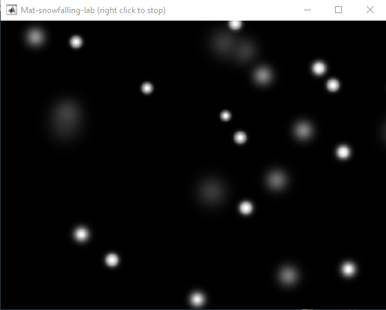
So I made this.
clear
close all
clc
% inspired from: https://www.youtube.com/watch?v=3CuUmy7jX6k
%% user parameters
h = 768;
w = 1024;
N_snowflakes = 50;
%% set figure window
figure(NumberTitle="off", ...
name='Mat-snowfalling-lab (right click to stop)', ...
MenuBar="none")
ax = gca;
ax.XAxisLocation = 'origin';
ax.YAxisLocation = 'origin';
axis equal
axis([0, w, 0, h])
ax.Color = 'k';
ax.XAxis.Visible = 'off';
ax.YAxis.Visible = 'off';
ax.Position = [0, 0, 1, 1];
%% first snowflake
ht = gobjects(1, 1);
for i=1:length(ht)
ht(i) = hgtransform();
ht(i).UserData = snowflake_factory(h, w);
ht(i).Matrix(2, 4) = ht(i).UserData.y;
ht(i).Matrix(1, 4) = ht(i).UserData.x;
im = imagesc(ht(i), ht(i).UserData.img);
im.AlphaData = ht(i).UserData.alpha;
colormap gray
end
%% falling snowflake
tic;
while true
% add a snowflake every 0.3 seconds
if toc > 0.3
if length(ht) < N_snowflakes
ht = [ht; hgtransform()];
ht(end).UserData = snowflake_factory(h, w);
ht(end).Matrix(2, 4) = ht(end).UserData.y;
ht(end).Matrix(1, 4) = ht(end).UserData.x;
im = imagesc(ht(end), ht(end).UserData.img);
im.AlphaData = ht(end).UserData.alpha;
colormap gray
end
tic;
end
ax.CLim = [0, 0.0005]; % prevent from auto clim
% move snowflakes
for i = 1:length(ht)
ht(i).Matrix(2, 4) = ht(i).Matrix(2, 4) + ht(i).UserData.velocity;
end
if strcmp(get(gcf, 'SelectionType'), 'alt')
set(gcf, 'SelectionType', 'normal')
break
end
drawnow
% delete the snowflakes outside the window
for i = length(ht):-1:1
if ht(i).Matrix(2, 4) < -length(ht(i).Children.CData)
delete(ht(i))
ht(i) = [];
end
end
end
%% snowflake factory
function snowflake = snowflake_factory(h, w)
radius = round(rand*h/3 + 10);
sigma = radius/6;
snowflake.velocity = -rand*0.5 - 0.1;
snowflake.x = rand*w;
snowflake.y = h - radius/3;
snowflake.img = fspecial('gaussian', [radius, radius], sigma);
snowflake.alpha = snowflake.img/max(max(snowflake.img));
end
Hello,
I have a MATLAB App that has been devolped in the MATLAB App Designer. I have saved all of the apps properties when the user selects the save config menu option and saved it into a .mat file.
Now I want to be able to load this file and update the app to the properties saved in this file. Currently, the program will store the variables in the app structure, but will not update the app's UIFigure. If I save the the UIFigure itself the program will create a new UIFigure and the code in App Designer will no longer work. Hence, why I've added not to save the UIFigure.
if strcmp(propName, 'SuperMarioUIFigure')
continue;
end
Does anyone know how I can get the app structure to update the current UIFigure that App Designer is running?
Here is my current code.
% Menu selected function: SaveConfigMenu
function SaveConfigMenuSelected(app, event)
% Create a structure to hold all the properties of the app
config = struct();
% List all properties of the app
metaProps = properties(app);
% Loop through properties and store their values in structure
for i = 1:length(metaProps)
propName = metaProps{i};
if strcmp(propName, 'SuperMarioUIFigure')
continue;
end
try
config.(propName) = app.(propName);
catch
% Handle any properties that can't be saved
fprintf('Could not save property: %s\n', propName);
end
end
% Prompt user to specify a file to save the configuration
[file, path] = uiputfile('*.mat', 'Save Configuration As');
if isequal(file, 0) || isequal(path, 0)
return; % User cancelled
end
% Save the configuration structure to a file
save(fullfile(path, file), '-struct', 'config');
uialert(app.SuperMarioUIFigure, 'Configuration saved successfully!', 'Save Configuration');
end
% Menu selected function: LoadConfigMenu
function LoadConfigMenuSelected(app, event)
% Prompt user to select a configuration file
[file, path] = uigetfile('*.mat', 'Load Configuration');
if isequal(file, 0) || isequal(path, 0)
return; % User cancelled
end
% Load the configuration structure from the file
config = load(fullfile(path, file));
% List all properties of the app
metaProps = properties(app);
% Update app properties with values from the configuration file
for i = 1:length(metaProps)
propName = metaProps{i};
if isfield(config, propName)
try
app.(propName) = config.(propName);
catch ME
% Handle any properties that can't be updated
fprintf('Could not load property: %s. Error: %s\n', propName, ME.message);
end
end
end
% Display a success message
uialert(app.SuperMarioUIFigure, 'Configuration loaded successfully!', 'Load Configuration');
end
Thanks
Hello, I have a very simple Simulink program to control a servo with my Arduino. The problem is that I'm not getting a full range of the servo. I am using an Adafruit Motor Shield to drive the servo which is a cheap TowerPro. The range I'm getting is 0 to 70. I am using Matlab/Simulink 2019.
Any ideas what could be wrong?
Thank you
The expression for a zero-symmetric polyhedron is known, S={x:[1; 1]<=Ax<=[1; 1]}, where A=[0.5 0; -0.5 0; 0 0.25; 0 -0.25], can you use the polyhedron function to draw an image of the polyhedron, I hope you can write detailed code
if app.LikeCheckBox.Value==true
app.EditField.Value='you Like our channal'
elseif app.LikeCheckBox.Value==true && app.ShareCheckBox.Value==true
app.EditField.Value='you liked and shared'
elseif app.ShareCheckBox.Value==true
app.EditField.Value='you Share our channal'
elseif app.ShareCheckBox.Value==true && app.SubscribeCheckBox.Value==true
app.EditField.Value='you shared and subscribed'
elseif app.SubscribeCheckBox.Value==true
app.EditField.Value='you Subscribed to our channal'
elseif app.LikeCheckBox.Value==true && app.SubscribeCheckBox.Value==true
app.EditField.Value='good job'
else app.EditField.Value='Choose on item'
app.EditField.HorizontalAlignment='center'
end
At the present time, the following problems are known in MATLAB Answers itself:
- Symbolic output is not displaying. The work-around is to disp(char(EXPRESSION)) or pretty(EXPRESSION)
- Symbolic preferences are sometimes set to non-defaults
Just shared an amazing YouTube video that demonstrates a real-time PID position control system using MATLAB and Arduino.
When I am inputting data, I am trying to input an equation that I should result in multiple answers. The equation I am trying to do is an output in Kw, divided by a conversion percentage. That percentage ranges from 5-15. No matter what way I put this data in to the system, it kicks out a bunch of 0's and then one column of real numners. The data chart should be 5 columns wide and 11 rows down, but for some reason it is giving me excess columns. 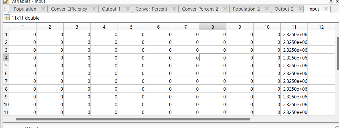
I don't like the change
16%
I really don't like the change
29%
I'm okay with the change
24%
I love the change
11%
I'm indifferent
11%
I want both the web & help browser
11%
38 票

You can make a lot of interesting objects with matlab primitive shapes (e.g. "cylinder," "sphere," "ellipsoid") by beginning with some of the built-in Matlab primitives and simply applying deformations. The gif above demonstrates how the Manta animation was created using a cylinder as the primitive and successively applying deformations: (https://www.mathworks.com/matlabcentral/communitycontests/contests/8/entries/16252);
Similarly, last year a sphere was deformed to create a face in two of my submissions, for example, the profile in "waking":
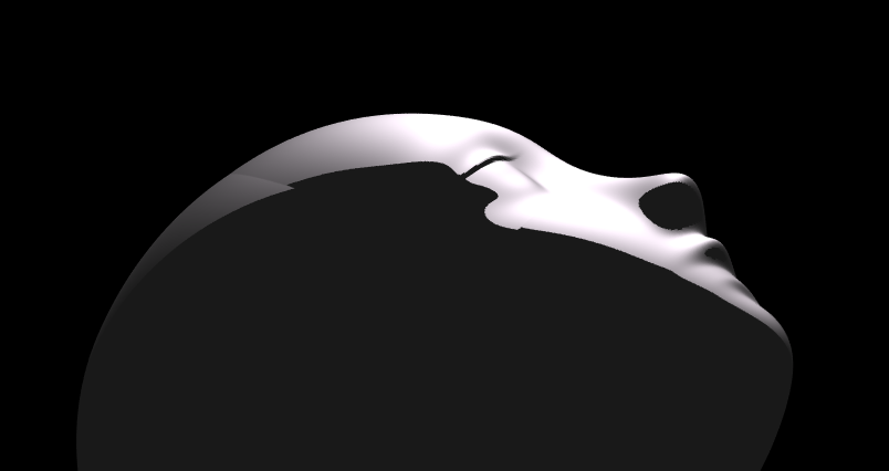
You can piece-wise assemble images, but one of the advantages of creating objects with deformations is that you have a parametric representation of the surface. Creating a higher or lower polygon rendering of the surface is as simple as declaring the number of faces in the orignal primitive. For example here is the scene in "snowfall" using sphere with different numbers of input faces:
sphere(100)
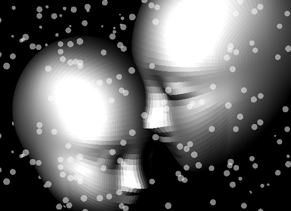
sphere(500)
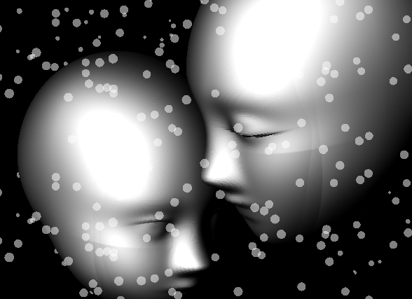
High poly models aren't always better. Low-polygon shapes can sometimes add a little distance from that low point in the uncanny valley.
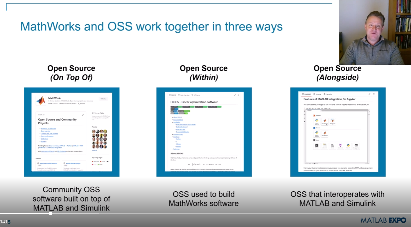
Next week is MATLAB EXPO week and it will be the first one that I'm presenting at! I'll be giving two presentations, both of which are related to the intersection of MATLAB and open source software.
- Open Source Software and MATLAB: Principles, Practices, and Python Along with MathWorks' Heather Gorr. We we discuss three different types of open source software with repsect to their relationship to MATLAB
- The CLASSIX Story: Developing the Same Algorithm in MATLAB and Python Simultaneously A collaboration with Prof. Stefan Guettel from University of Manchester. Developing his clustering algorithm, CLASSIX, in both Python and MATLAB simulatenously helped provide insights that made the final code better than if just one language was used.
There are a ton of other great talks too. Come join us! (It's free!) MATLAB EXPO 2024
Hi MATLAB Central community! 👋
I’m currently working on a project where I’m integrating MATLAB analytics into a mobile app, mainly to handle data-heavy tasks like processing sensor data and running predictive models. The app is built for Android, and while it’s not entirely MATLAB-based, I use MATLAB for a lot of data preprocessing and model training.
I wanted to reach out and see if anyone else here has experience with using MATLAB for similar mobile or embedded applications. Here are a few areas I’m focusing on:1. Optimizing MATLAB Code for Mobile Compatibility
I’ve found that some MATLAB functions work perfectly on desktop but may run slower or encounter limitations on mobile. I’ve tried using code generation and reducing function calls where possible, but I’m curious if anyone has other tips for optimizing MATLAB code for mobile environments?
2. Using MATLAB for Sensor Data Processing
I’m working with accelerometer and GPS data, and MATLAB has been great for preprocessing. However, I wonder if anyone has suggestions for handling large sensor datasets efficiently in MATLAB, especially if you've managed data in mobile contexts?
3. Integrating MATLAB Models into Mobile Apps
I’ve heard about using MATLAB Compiler SDK to integrate MATLAB algorithms into other environments. For those who have done this, what’s the best way to maintain performance without excessive computational strain on the device?
4. Data Visualization Tips
Has anyone had experience with mobile-friendly data visualizations using MATLAB? I’ve been using basic plots, but I’d love to know if there are any resources or toolboxes that make it easier to create lightweight, interactive visuals for mobile.
If anyone here has tips, tools, or experiences with MATLAB in mobile development, I’d love to hear them! Thanks in advance for any advice you can share!
It would be nice to have a function to shade between two curves. This is a common question asked on Answers and there are some File Exchange entries on it but it's such a common thing to want to do I think there should be a built in function for it. I'm thinking of something like
plotsWithShading(x1, y1, 'r-', x2, y2, 'b-', 'ShadingColor', [.7, .5, .3], 'Opacity', 0.5);
So we can specify the coordinates of the two curves, and the shading color to be used, and its opacity, and it would shade the region between the two curves where the x ranges overlap. Other options should also be accepted, like line with, line style, markers or not, etc. Perhaps all those options could be put into a structure as fields, like
plotsWithShading(x1, y1, options1, x2, y2, options2, 'ShadingColor', [.7, .5, .3], 'Opacity', 0.5);
the shading options could also (optionally) be a structure. I know it can be done with a series of other functions like patch or fill, but it's kind of tricky and not obvious as we can see from the number of questions about how to do it.
Does anyone else think this would be a convenient function to add?
My favorite image processing book is The Image Processing Handbook by John Russ. It shows a wide variety of examples of algorithms from a wide variety of image sources and techniques. It's light on math so it's easy to read. You can find both hardcover and eBooks on Amazon.com Image Processing Handbook
There is also a Book by Steve Eddins, former leader of the image processing team at Mathworks. Has MATLAB code with it. Digital Image Processing Using MATLAB
You might also want to look at the free online book http://szeliski.org/Book/
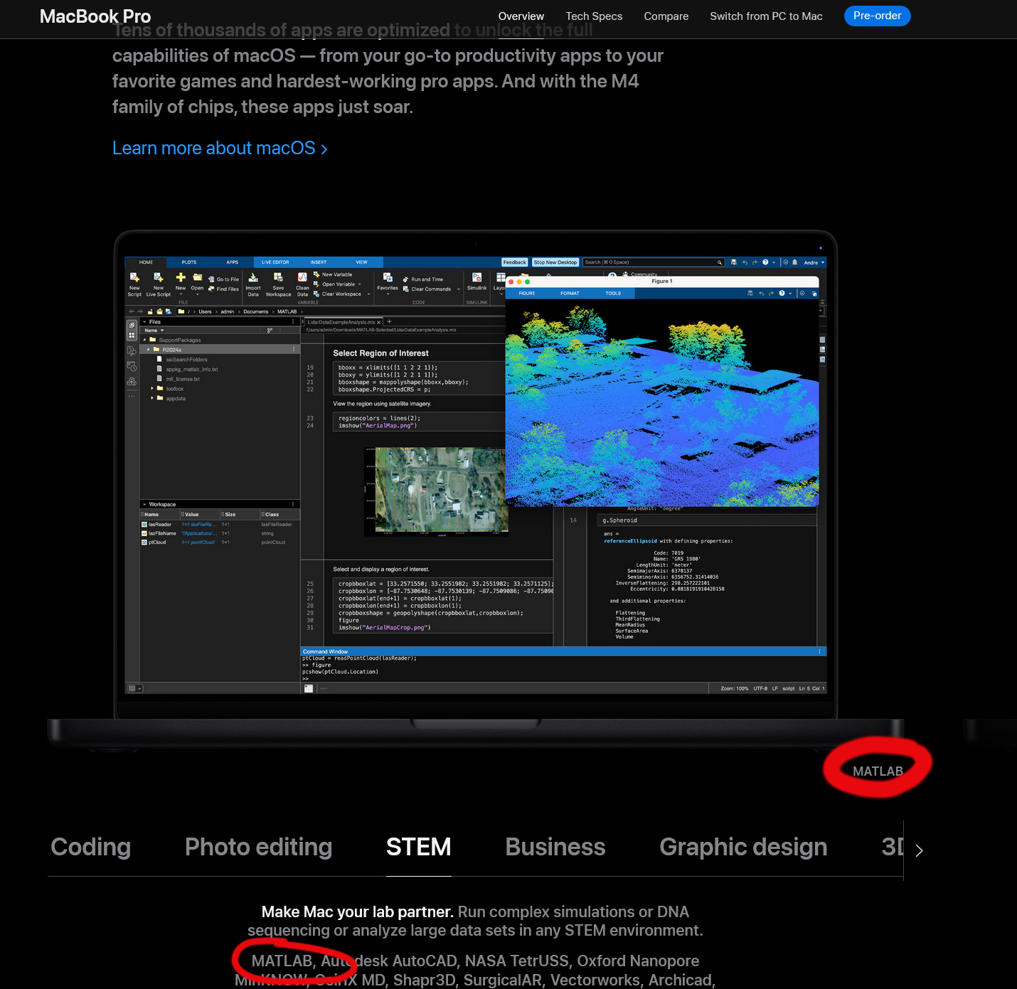
Go to this page, scroll down to the middle of the long page where you see "Coding Photo editing STEM Business ...." and select "STEM". Voilà!
In the past two years, large language models have brought us significant changes, leading to the emergence of programming tools such as GitHub Copilot, Tabnine, Kite, CodeGPT, Replit, Cursor, and many others. Most of these tools support code writing by providing auto-completion, prompts, and suggestions, and they can be easily integrated with various IDEs.
As far as I know, aside from the MATLAB-VSCode/MatGPT plugin, MATLAB lacks such AI assistant plugins for its native MATLAB-Desktop, although it can leverage other third-party plugins for intelligent programming assistance. There is hope for a native tool of this kind to be built-in.
Mini Hack is brilliant!Let's use MATLAB to create the future!
Pumpkins have been a popular, recurring, and ever-evolving theme in MATLAB during the past few years, and particularly during this time of year. Much of this is driven by the epic work of @Eric Ludlam and expanded upon by many others. The list of material is too extensive to go through everything individually, but I'm listing some of my favourite resources below and I highly recommend these to everyone as they're a lot of fun to play with:
Pumpkins are also particularly prominent during the yearly Mini Hack Contests. This year, I have jumped onto the bandwagon myself with my Floating Pumpkins entry:
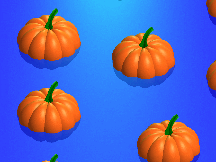
In this post, I would like to introduce the concept of masking 3D surfaces in a festive and fun way, by showcasing how to apply it for carving faces on pumpkins step by step.
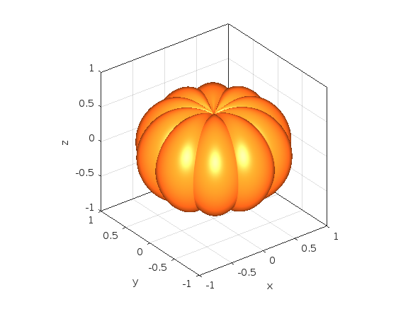
Let's start by drawing the pumpkin's body. The following was adapted from Eric's code:
n = 600; % Number of faces
% Shape pumpkin's rind (skin)
[X,Y,Z] = sphere(n);
% Shape pumpkin's ribs (ridges)
R = (1-(1-mod(0:20/n:20,2)).^2/12);
X = X.*R; Y = Y.*R; Z = Z.*R;
Z = (.8+(0-linspace(1,-1,n+1)'.^4)*.3).*Z;
function plotPumpkin(X,Y,Z)
figure
surf(X,Y,Z,'FaceColor',[1 .4 .1],'EdgeColor','none');
hold on
box on
axis([-1 1 -1 1 -1 1],'square')
xlabel('x'); xticks(-1:0.5:1)
ylabel('y'); yticks(-1:0.5:1)
zlabel('z'); zticks(-1:0.5:1)
material([.45,.7,.25])
camlight('headlight')
camlight('headlight')
lighting gouraud
end
plotPumpkin(X,Y,Z)
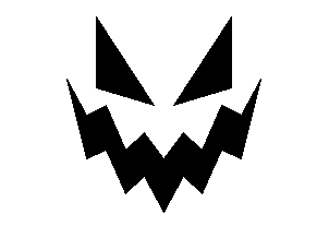
The next step is drawing the face for the mask. This can be done in 2D and can consist of any number of lines that form polygonal closed shapes and are appropriately scaled relative to the coordinates of the pumpkin. A quick example:
% Mouth
xm = [-.5:.1:.5 flip(-.5:.1:.5)];
ym = [.15 -.3 -.25 -.5 -.4 -.6 flip([.15 -.3 -.25 -.5 -.4]) .15 -.05 0 -.25 -.15 -.3 flip([.15 -.05 0 -.25 -.15])];
% Right eye
xr = [-.35 -.05 -.35];
yr = [.1 0 .5];
% Left eye
xl = abs(xr);
yl = yr;
figure('Color','w')
set(gcf,'Position',get(gcf,'Position')/2)
axes('Visible','off','NextPlot','Add')
axis tight square
fill(xm,ym,'k')
fill(xr,yr,'k')
fill(xl,yl,'k')
We then need to apply the 2D mask to the 3D surface. To do that, we project it onto the intersections of the surface with the XY plane. However, as we need the face to appear on the side of the pumpkin, we first need to rotate the pumpkin so that the front side is facing upwards. Essentially, we need to rotate the pumpkin around the x-axis by -π/2 rad.
Let's do this from first principles to better understand the process:
theta = [-pi/2,0,0];
[X,Y,Z] = xyzRotate(X,Y,Z,theta);
function [X,Y,Z] = xyzRotate(X,Y,Z,theta)
% Rotation matrices
Rx = [1 0 0;0 cos(theta(1)) -sin(theta(1));0 sin(theta(1)) cos(theta(1))];
Ry = [cos(theta(2)) 0 sin(theta(2));0 1 0;-sin(theta(2)) 0 cos(theta(2))];
Rz = [cos(theta(3)) -sin(theta(3)) 0;sin(theta(3)) cos(theta(3)) 0;0 0 1];
for i=1:size(X,1)
for j=1:size(X,2)
r=Rx*Ry*Rz*[X(i,j);Y(i,j);Z(i,j)];
X(i,j)=r(1);
Y(i,j)=r(2);
Z(i,j)=r(3);
end
end
end
More information about these transformations can be found here:
When plotting we get:
plotPumpkin(X,Y,Z)
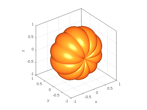
Note that as we have only rotated this around the x-axis, Ry and Rz are equal to eye(3).
We can now apply the mask as discussed. We do this by using one of my favourite functions inpolygon. This gives us the corresponding indices of all the data points located inside our polygonal regions. At this stage, it's important to keep the following in mind:
- The number of faces (n) controls the discretization of the pumpkin. The larger it is, the smoother the mask will be, but at the same time the computational cost will also increase. If you are using this for the contest which has a timeout limit of 235 seconds, you might need to adjust it accordingly.
- You will also need to restrict the Z-coordinates appropriately (Z>=0) so that the mask is only applied on the front side of the pumpkin.
- If you are animating the face mask (more information about this below), and you need the eyes and mouth to fully close at any point, avoid using the second argument of the inpolygon function that gives you the points located on the edge of the regions.
The masking function is given below:
function [X,Y,Z] = Mask(X,Y,Z,xm,ym,xr,yr,xl,yl)
mask = ones(size(Z));
mask((inpolygon(X,Y,xm,ym)|inpolygon(X,Y,xr,yr)|inpolygon(X,Y,xl,yl))&Z>=0) = NaN;
Z = Z.*mask;
end
Applying the mask gives us:
[X,Y,Z]=Mask(X,Y,Z,xm,ym,xr,yr,xl,yl);
plotPumpkin(X,Y,Z)
arrayfun(@(x)light('style','local','position',[0 0 0],'color','y'),1:2)
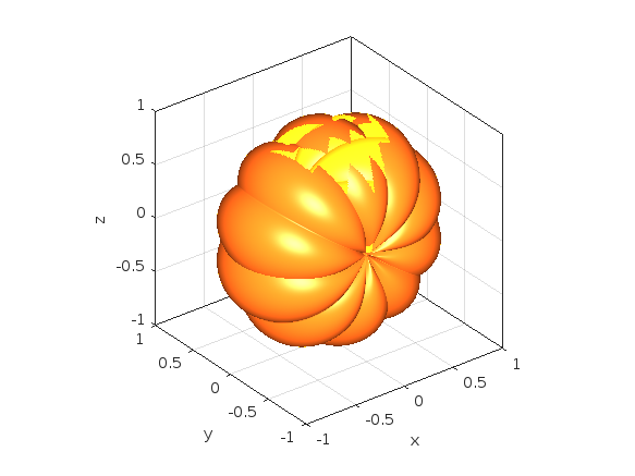
We can see that MATLAB was thoughtful enough to automatically remove the pulp from inside the pumpkin, proving its convenience time and time again.
We can then rotate the pumpkin back and add the stem to get the final result:
theta = [pi/2,0,0];
[X,Y,Z] = xyzRotate(X,Y,Z,theta);
% Stem
s = [1.5 1 repelem(.7, 6)] .* [repmat([.1 .06],1,round(n/20)) .1]';
[t,p] = meshgrid(0:pi/15:pi/2,linspace(0,pi,round(n/10)+1));
Xs = repmat(-(.4-cos(p).*s).*cos(t)+.4,2,1);
Ys = [-sin(p).*s;sin(p).*s];
Zs = repmat((.5-cos(p).*s).*sin(t)+.55,2,1);
plotPumpkin(X,Y,Z)
arrayfun(@(x)light('style','local','position',[0 0 0],'color','y'),1:2)
surf(Xs,Ys,Zs,'FaceColor','#008000','EdgeColor','none');
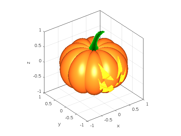
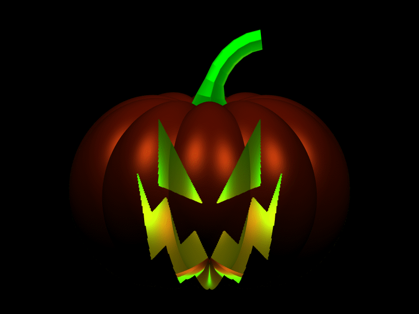
And that's it. You can now add some change to the mask's coordinates between frames and play around with the lighting to get results such as these (more information on how to do this on my Teaser entry):

I hope you have found this tutorial useful, and I'm looking forward to seeing many more creative entries during the final week of the contest.