結果:
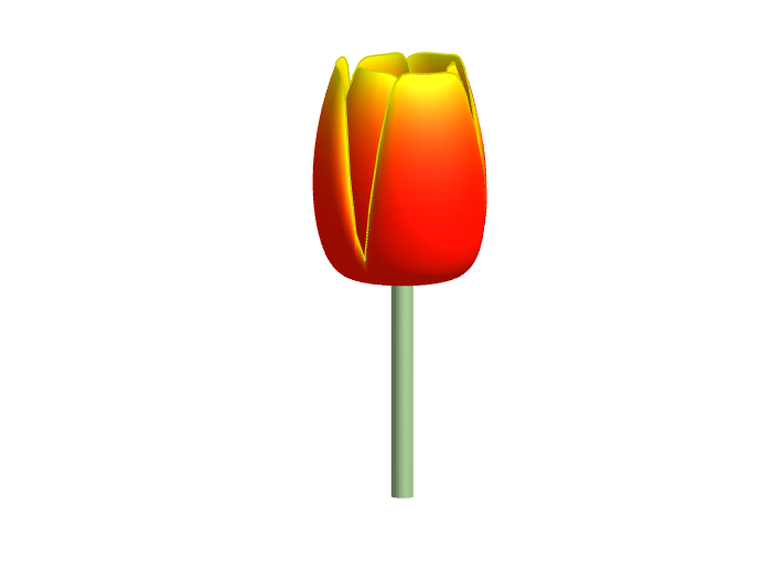
Spring is here in Natick and the tulips are blooming! While tulips appear only briefly here in Massachusetts, they provide a lot of bright and diverse colors and shapes. To celebrate this cheerful flower, here's some code to create your own tulip!
Check out this episode about PIVLab: https://www.buzzsprout.com/2107763/15106425
Join the conversation with William Thielicke, the developer of PIVlab, as he shares insights into the world of particle image velocimetery (PIV) and its applications. Discover how PIV accurately measures fluid velocities, non invasively revolutionising research across the industries. Delve into the development journey of PI lab, including collaborations, key features and future advancements for aerodynamic studies, explore the advanced hardware setups camera technologies, and educational prospects offered by PIVlab, for enhanced fluid velocity measurements. If you are interested in the hardware he speaks of check out the company: Optolution.
One of the starter prompts is about rolling two six-sided dice and plot the results. As a hobby, I create my own board games. I was able to use the dice rolling prompt to show how a simple roll and move game would work. That was a great surprise!
How to leave feedback on a doc page
Leaving feedback is a two-step process. At the bottom of most pages in the MATLAB documentation is a star rating.

Start by selecting a star that best answers the question. After selecting a star rating, an edit box appears where you can offer specific feedback.

When you press "Submit" you'll see the confirmation dialog below. You cannot go back and edit your content, although you can refresh the page to go through that process again.

Tips on leaving feedback
- Be productive. The reader should clearly understand what action you'd like to see, what was unclear, what you think needs work, or what areas were really helpful.
- Positive feedback is also helpful. By nature, feedback often focuses on suggestions for changes but it also helps to know what was clear and what worked well.
- Point to specific areas of the page. This helps the reader to narrow the focus of the page to the area described by your feedback.
What happens to that feedback?
Before working at MathWorks I often left feedback on documentation pages but I never knew what happens after that. One day in 2021 I shared my speculation on the process:
> That feedback is received by MathWorks Gnomes which are never seen nor heard but visit the MathWorks documentation team at night while they are sleeping and whisper selected suggestions into their ears to manipulate their dreams. Occassionally this causes them to wake up with a Eureka moment that leads to changes in the documentation.

I'd like to let you in on the secret which is much less fanciful. Feedback left in the star rating and edit box are collected and periodically reviewed by the doc writers who look for trends on highly trafficked pages and finer grain feedback on less visited pages. Your feedback is important and often results in improvements.
Let's talk about probability theory in Matlab.
Conditions of the problem - how many more letters do I need to write to the sales department to get an answer?
To get closer to the problem, I need to buy a license under a contract. Maybe sometimes there are responsible employees sitting here who will give me an answer.
Thank you
In the MATLAB description of the algorithm for Lyapunov exponents, I believe there is ambiguity and misuse.
The lambda(i) in the reference literature signifies the Lyapunov exponent of the entire phase space data after expanding by i time steps, but in the calculation formula provided in the MATLAB help documentation, Y_(i+K) represents the data point at the i-th point in the reconstructed data Y after K steps, and this calculation formula also does not match the calculation code given by MATLAB. I believe there should be some misguidance and misunderstanding here.
According to the symbol regulations in the algorithm description and the MATLAB code, I think the correct formula might be y(i) = 1/dt * 1/N * sum_j( log( ||Y_(j+i) - Y_(j*+i)|| ) )
Cordial saludo , Necesito simular un generador electrico que tiene una entrada mecanica y genera el suficiente voltage y corriente para encender un LED.
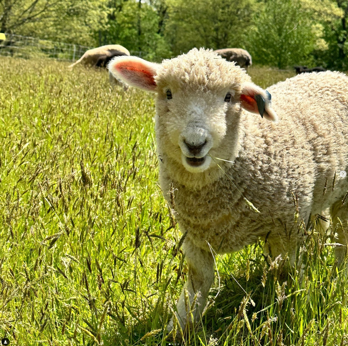
Drumlin Farm has welcomed MATLAMB, named in honor of MathWorks, among ten adorable new lambs this season!
A colleague said that you can search the Help Center using the phrase 'Introduced in' followed by a release version. Such as, 'Introduced in R2022a'. Doing this yeilds search results specific for that release.
Seems pretty handy so I thought I'd share.
Are you local to Boston?
Shape the Future of MATLAB: Join MathWorks' UX Night In-Person!
When: June 25th, 6 to 8 PM
Where: MathWorks Campus in Natick, MA
🌟 Calling All MATLAB Users! Here's your unique chance to influence the next wave of innovations in MATLAB and engineering software. MathWorks invites you to participate in our special after-hours usability studies. Dive deep into the latest MATLAB features, share your valuable feedback, and help us refine our solutions to better meet your needs.
🚀 This Opportunity Is Not to Be Missed:
- Exclusive Hands-On Experience: Be among the first to explore new MATLAB features and capabilities.
- Voice Your Expertise: Share your insights and suggestions directly with MathWorks developers.
- Learn, Discover, and Grow: Expand your MATLAB knowledge and skills through firsthand experience with unreleased features.
- Network Over Dinner: Enjoy a complimentary dinner with fellow MATLAB enthusiasts and the MathWorks team. It's a perfect opportunity to connect, share experiences, and network after work.
- Earn Rewards: Participants will not only contribute to the advancement of MATLAB but will also be compensated for their time. Plus, enjoy special MathWorks swag as a token of our appreciation!
👉 Reserve Your Spot Now: Space is limited for these after-hours sessions. If you're passionate about MATLAB and eager to contribute to its development, we'd love to hear from you.

Bringing the beauty of MathWorks Natick's tulips to life through code!
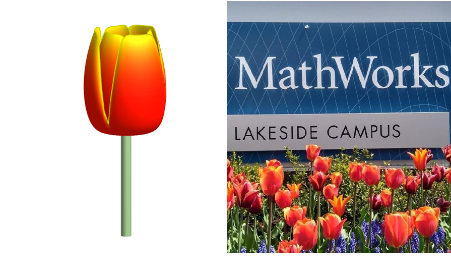
Remix challenge: create and share with us your new breeds of MATLAB tulips!
Hello MATLAB community,
I am doing some image processing with MATLAB and some issues with my coding. I just like to warn you that I am very new at coding and MATLAB so I apologise in advance for my low level and I would be very glad to have some help as I have hitted a wall, and can't find a solution to my problem.
Context: I have a video of beams, that move right to left over time. The base is fixed, only the beam moves. I converted the video to images, and my MATLAB program is going through the image file and treating every image in it. Here are two image examples:
 and
and 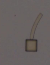
I want to measure the following things:
a. The coordinates between the 2 extremities of the beam (length of the beam, without its base), let's call them A and B.
b. The bending deformation E (L0-Lt/L0 *100), obtained by calculating the distance between A and B, called Lt.
c. the curvature of the beam (1/R), obtained by extracting the radius R of a circle fitting the curvature of the beam.
d. The angle between a vertical line passing through A, and the line AB.
What I have done so far:
My approach has been to transform my image into an rgbimage, then binaryImage, then have the complementary image, apply some modifications/corrections to the image, and then skeletonize it. And from then, I extract the coordinates of A and B, the distance between A&B (Lt), the radius of the beam R, and the angle between A&B (T).
My main issue is the skeletonisation. Because my beam is quite thick, it shortens up too much my beam, and in an inconcistent manner. So then my results are completly wrong. Here is an image of the different images and operation I have done and the result:
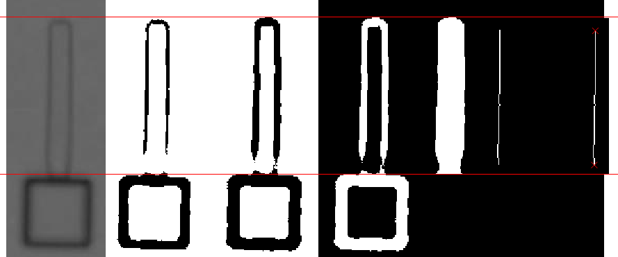
So as you can see, the length is shorter. I would like to have a skeleton that meets the edges of the beam to calculate the end points.
I have tried "bwskel(BW, 'MinBranchLength', 30)" and "bwmorph(BW, 'thin', inf)", and this: https://uk.mathworks.com/matlabcentral/fileexchange/11123-better-skeletonization. But the problem remains the same. I have tried regionpropos, but the major axis they return is too long, I have tried bwferet(), but the maxlength is in diagonal of the beam... I have running out of ideas.
Problem: So I guess my main problem is how can I get a skeletonisation that goes to the edges of the beam?
Here is my code:
for i = TrackingStart:TrackingEnd
FileRGB(:,:,i) = rgb2gray(imread(IMG)); % Convert to grayscale
croppedRGB = FileRGB(y3left:y3right, x3left:x3right, i);
binaryImage = imbinarize(croppedRGB, 'adaptive', 'ForegroundPolarity','dark','Sensitivity', 0.50);
out = nnz(~binaryImage);
while out <= 4300 % Change threshold if needed
for j = 1:50
sensitivity = 0.50 + j * 0.01;
binaryImage = imbinarize(croppedRGB, 'adaptive', 'ForegroundPolarity', 'dark', 'Sensitivity', sensitivity);
out = nnz(~binaryImage);
if out >= 4325
break; % Exit the loop if the condition is met
end
end
end
% Create a line Model
BW = imcomplement(binaryImage);
BW(y1left:y1right, x1left:x1right) = 1; % there is always sample at the junction area (between beam and base)
BW(y2left:y2right, x2left:x2right) = 0; % Always = 0 if no sample here
BW = bwmorph(BW, 'close', Inf);
BW = bwmorph(BW, 'bridge');
BW = bwareafilt(BW, 1);
s = regionprops(BW, 'FilledImage');
BW = s.FilledImage;
BW = bwskel(BW, 'MinBranchLength', 30);
endpoints = bwmorph(BW, 'endpoints');
[y_end, x_end] = find(endpoints == 1);
%Degree of bending deformation method
Lt = sqrt(power(x_end(1)-x_end(2),2)+power(y_end(1)-y_end(2),2));
if x_end(2) > x_end(1)
Lt = -Lt;
end
Lstore(i) = Lt;
%Curvature method
[row_dots_cir, col_dots_cir, val] = find(BW == 1);
[xc(i),yc(i),Rstore(i),a] = circfit(col_dots_cir,row_dots_cir);
%Angle method
slope_endpoints = (x_end(1) - x_end(2)) / (y_end(1) - y_end(2));
angle_radians = atan(slope_endpoints);
angle_degrees = rad2deg(angle_radians);
if x_end(2) > x_end(1)
angle_degrees = -angle_degrees;
end
Tstore(i) = angle_degrees;
i
end
I found this plot of words said by different characters on the US version of The Office sitcom. There's a sparkline for each character from pilot to finale episode.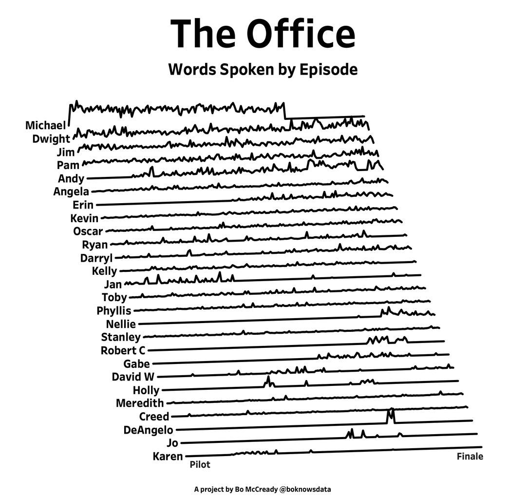
A high school student called for help with this physics problem:
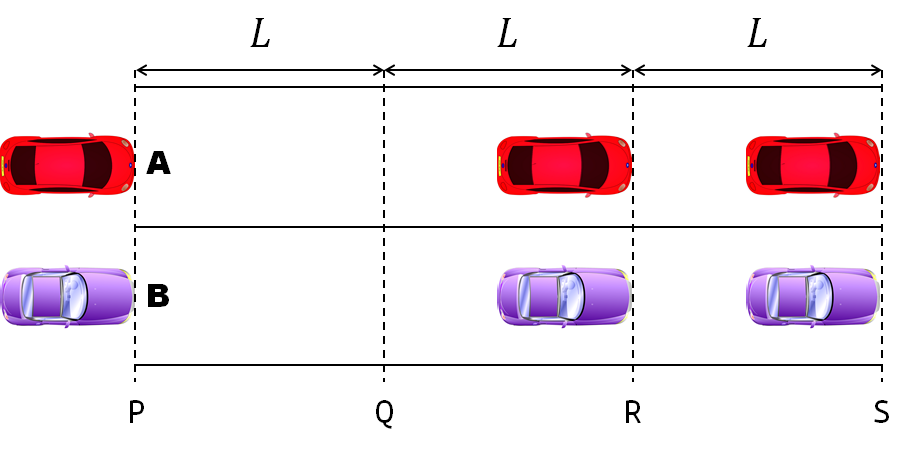
- Car A moves with constant velocity v.
- Car B starts to move when Car A passes through the point P.
- Car B undergoes...
- uniform acc. motion from P to Q.
- uniform velocity motion from Q to R.
- uniform acc. motion from R to S.
- Car A and B pass through the point R simultaneously.
- Car A and B arrive at the point S simultaneously.
Q1. When car A passes the point Q, which is moving faster?
Q2. Solve the time duration for car B to move from P to Q using L and v.
Q3. Magnitude of acc. of car B from P to Q, and from R to S: which is bigger?
Well, it can be solved with a series of tedious equations. But... how about this?
Code below:
%% get images and prepare stuffs
figure(WindowStyle="docked"),
ax1 = subplot(2,1,1);
hold on, box on
ax1.XTick = [];
ax1.YTick = [];
A = plot(0, 1, 'ro', MarkerSize=10, MarkerFaceColor='r');
B = plot(0, 0, 'bo', MarkerSize=10, MarkerFaceColor='b');
[carA, ~, alphaA] = imread('https://cdn.pixabay.com/photo/2013/07/12/11/58/car-145008_960_720.png');
[carB, ~, alphaB] = imread('https://cdn.pixabay.com/photo/2014/04/03/10/54/car-311712_960_720.png');
carA = imrotate(imresize(carA, 0.1), -90);
carB = imrotate(imresize(carB, 0.1), 180);
alphaA = imrotate(imresize(alphaA, 0.1), -90);
alphaB = imrotate(imresize(alphaB, 0.1), 180);
carA = imagesc(carA, AlphaData=alphaA, XData=[-0.1, 0.1], YData=[0.9, 1.1]);
carB = imagesc(carB, AlphaData=alphaB, XData=[-0.1, 0.1], YData=[-0.1, 0.1]);
txtA = text(0, 0.85, 'A', FontSize=12);
txtB = text(0, 0.17, 'B', FontSize=12);
yline(1, 'r--')
yline(0, 'b--')
xline(1, 'k--')
xline(2, 'k--')
text(1, -0.2, 'Q', FontSize=20, HorizontalAlignment='center')
text(2, -0.2, 'R', FontSize=20, HorizontalAlignment='center')
% legend('A', 'B') % this make the animation slow. why?
xlim([0, 3])
ylim([-.3, 1.3])
%% axes2: plots velocity graph
ax2 = subplot(2,1,2);
box on, hold on
xlabel('t'), ylabel('v')
vA = plot(0, 1, 'r.-');
vB = plot(0, 0, 'b.-');
xline(1, 'k--')
xline(2, 'k--')
xlim([0, 3])
ylim([-.3, 1.8])
p1 = patch([0, 0, 0, 0], [0, 1, 1, 0], [248, 209, 188]/255, ...
EdgeColor = 'none', ...
FaceAlpha = 0.3);
%% solution
v = 1; % car A moves with constant speed.
L = 1; % distances of P-Q, Q-R, R-S
% acc. of car B for three intervals
a(1) = 9*v^2/8/L;
a(2) = 0;
a(3) = -1;
t_BatQ = sqrt(2*L/a(1)); % time when car B arrives at Q
v_B2 = a(1) * t_BatQ; % speed of car B between Q-R
%% patches for velocity graph
p2 = patch([t_BatQ, t_BatQ, t_BatQ, t_BatQ], [1, 1, v_B2, v_B2], ...
[248, 209, 188]/255, ...
EdgeColor = 'none', ...
FaceAlpha = 0.3);
p3 = patch([2, 2, 2, 2], [1, v_B2, v_B2, 1], [194, 234, 179]/255, ...
EdgeColor = 'none', ...
FaceAlpha = 0.3);
%% animation
tt = linspace(0, 3, 2000);
for t = tt
A.XData = v * t;
vA.XData = [vA.XData, t];
vA.YData = [vA.YData, 1];
if t < t_BatQ
B.XData = 1/2 * a(1) * t^2;
vB.XData = [vB.XData, t];
vB.YData = [vB.YData, a(1) * t];
p1.XData = [0, t, t, 0];
p1.YData = [0, vB.YData(end), 1, 1];
elseif t >= t_BatQ && t < 2
B.XData = L + (t - t_BatQ) * v_B2;
vB.XData = [vB.XData, t];
vB.YData = [vB.YData, v_B2];
p2.XData = [t_BatQ, t, t, t_BatQ];
p2.YData = [1, 1, vB.YData(end), vB.YData(end)];
else
B.XData = 2*L + v_B2 * (t - 2) + 1/2 * a(3) * (t-2)^2;
vB.XData = [vB.XData, t];
vB.YData = [vB.YData, v_B2 + a(3) * (t - 2)];
p3.XData = [2, t, t, 2];
p3.YData = [1, 1, vB.YData(end), v_B2];
end
txtA.Position(1) = A.XData(end);
txtB.Position(1) = B.XData(end);
carA.XData = A.XData(end) + [-.1, .1];
carB.XData = B.XData(end) + [-.1, .1];
drawnow
end
I have question about using 'bnlssm' object when the problem involves time-varying coefs. Per this documentation https://www.mathworks.com/help/econ/bnlssm.html , bnlssm allows the transition matrix to be a nonlinear function of the past values of the state vector, while also being time-varying --, i.e. A_t(x_{t-1}). However the documentation contains an example of the parameter mapping function for a fixed coef. case only:
function [A,B,C,D,Mean0,Cov0,StateType] = paramMap(theta)
A = @(x)blkdiag([theta(1) theta(2); 0 1],[theta(3) theta(4); 0 1])*x;
B = [theta(5) 0; 0 0; 0 theta(6); 0 0];
C = @(x)log(exp(x(1)-theta(2)/(1-theta(1))) + ...
exp(x(3)-theta(4)/(1-theta(3))));
D = theta(7);
Mean0 = [theta(2)/(1-theta(1)); 1; theta(4)/(1-theta(3)); 1];
Cov0 = diag([theta(5)^2/(1-theta(1)^2) 0 theta(6)^2/(1-theta(3)^2) 0]);
StateType = [0; 1; 0; 1]; % Stationary state and constant 1 processes
end
Here, A and C are recognised as function handles and show the dimension of 1-by-1 when [A,B,C,D]=paramMap(theta) is run with a given theta. This does not prevent filter/smooth from returning the states estimates, as the function handles become m-by-m matices when the function handles are evaluated.
However, whenever I try replaceing A with a cell array, e.g.:
A=cell(T,1);
for t=1:T
A{t} = @(x)blkdiag([theta(1) theta(2); 0 1],[theta(3) theta(4); 0 1])*x;
end
bnlssm.fixcoeff throws an error that the dimensions of Mean0 are expected to be 1, per validation step in lines 700-707 of 'bnlssm.m':
if iscellA; At = A{1};
else; At = A; end
numStates0 = size(At,2);
if
isscalar(mean0)
mean0 = mean0(ones(numStates0,1),:);
elseif
~isempty(mean0)
mean0 = mean0(:);
validateattributes(mean0,{'numeric'},{'finite','real','numel',numStates0},callerName,'Mean0');
end
Q: Is it just overlook by MathWorks programmers and creating local verions of bnlssm/filter/smooth with that validation step removed is a viable pathway forward, or is it intentional because 'bnlssm' was in fact designed to handle only the time-invariant coef. case correctly?
is there any sites available online free ai course learning except: coursera.org
%%https://in.mathworks.com/matlabcentral/cody/problems/3-find-the-sum-of-all-the-numbers-of-the-input-vector/solutions/new#
%Above is the complete link of question that is ask and below i am providing my code for %this problem, please guide how do i rearrange this so that i can pass all the test at a time.
function y = vecsum(x)
x= 1:100;
y1= sum(x(1,[1]));
y2= sum(x(1,[1 2 3 5]));
y3= sum(x);
y=[y1 y2 y3];
end
Are you a Simulink user eager to learn how to create apps with App Designer? Or an App Designer enthusiast looking to dive into Simulink?
Don't miss today's article on the Graphics and App Building Blog by @Robert Philbrick! Discover how to build Simulink Apps with App Designer, streamlining control of your simulations!
Hi All,
I'm trying to get code coverage analysis report while cosimulation of generated HDL code through Questasim in Simulink. I'm getting blank results in coverage analysis section of Questasim. Can you please help me to get code coverage details ? Thanks in Advance.
Matlab: 2022b
Questasim: 2020.1