結果:
Hi,
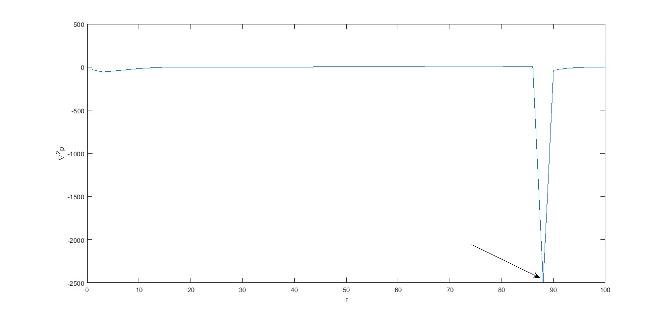
I have a plot as attached herewith in which the value of the point as shown by arrow mark is to be determined and compared to a reference value. It is plotted at a time step of 999 (t ranges from 1 to 1000).
global data;
cp=0;
for i=999:max(length(data.variable.t))
for j=60:max(length(data.variable.x))-1
if data.variable.curvepressure(i,j) <= -10.2661
disp(data.variable.curvepressure(i,j))
cp=1;
break
end
end
end
The above code is not working and need your advice please.
hello i found the following tools helpful to write matlab programs. copilot.microsoft.com chatgpt.com/gpts gemini.google.com and ai.meta.com. thanks a lot and best wishes.
Hi everyone,
I've recently joined a forest protection team in Greece, where we use drones for various tasks. This has sparked my interest in drone programming, and I'd like to learn more about it. Can anyone recommend any beginner-friendly courses or programs that teach drone programming?
I'm particularly interested in courses that focus on practical applications and might align with the work we do in forest protection. Any suggestions or guidance would be greatly appreciated!
Thank you!
I have picked the title but don't know which direction to take it. Looking for any and all inspiration. I took the project as it sounded interesting when reading into it, but I'm a satellite novice, and my degree is in electronics.
"What are your favorite features or functionalities in MATLAB, and how have they positively impacted your projects or research? Any tips or tricks to share?
Check out the LLMs with MATLAB project on File Exchange to access Large Language Models from MATLAB.
Along with the latest support for GPT-4o mini, you can use LLMs with MATLAB to generate images, categorize data, and provide semantic analyis.
function ans = your_fcn_name(n)
n;
j=sum(1:n);
a=zeros(1,j);
for i=1:n
a(1,((sum(1:(i-1))+1)):(sum(1:(i-1))+i))=i.*ones(1,i);
end
disp
Gabriel's horn is a shape with the paradoxical property that it has infinite surface area, but a finite volume.
Gabriel’s horn is formed by taking the graph of  with the domain
  and rotating it in three dimensions about the
  axis.
axis.
There is a standard formula for calculating the volume of this shape, for a general function  .Wwe will just state that the volume of the
  solid between a and b is:
The surface area of the solid is given by:
One other thing we need to consider is that we are trying to find the value of these integrals between 1 and ∞. An integral with a limit of infinity is called an improper integral and we can't evaluate it simply by plugging the value infinity into the normal equation for a definite integral. Instead, we must first calculate the definite integral up to some finite limit b and then calculate the limit of the result as b tends to ∞:
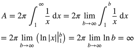
Volume
We can calculate the horn's volume using the volume integral above, so
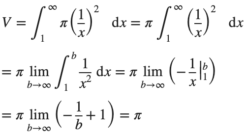
The total volume of this infinitely long trumpet isπ.
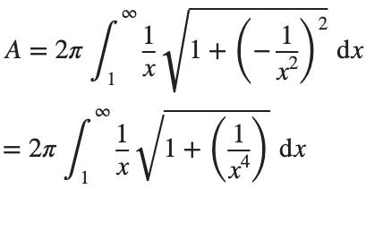
Surface Area
To determine the surface area, we first need the function’s derivative:
Now plug it into the surface area formula and we have:
This is an improper integral and it's hard to evaluate, but since in our interval 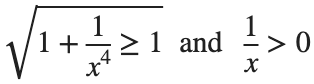
So, we have :
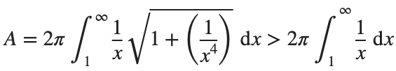
Now,we evaluate this last integral
So the surface are is infinite.
% Define the function for Gabriel's Horn
gabriels_horn = @(x) 1 ./ x;
% Create a range of x values
x = linspace(1, 40, 4000); % Increase the number of points for better accuracy
y = gabriels_horn(x);
% Create the meshgrid
theta = linspace(0, 2 * pi, 6000); % Increase theta points for a smoother surface
[X, T] = meshgrid(x, theta);
Y = gabriels_horn(X) .* cos(T);
Z = gabriels_horn(X) .* sin(T);
% Plot the surface of Gabriel's Horn
figure('Position', [200, 100, 1200, 900]);
surf(X, Y, Z, 'EdgeColor', 'none', 'FaceAlpha', 0.9);
hold on;
% Plot the central axis
plot3(x, zeros(size(x)), zeros(size(x)), 'r', 'LineWidth', 2);
% Set labels
xlabel('x');
ylabel('y');
zlabel('z');
% Adjust colormap and axis properties
colormap('gray');
shading interp; % Smooth shading
% Adjust the view
view(3);
axis tight;
grid on;
% Add formulas as text annotations
dim1 = [0.4 0.7 0.3 0.2];
annotation('textbox',dim1,'String',{'$$V = \pi \int_{1}^{a} \left( \frac{1}{x} \right)^2 dx = \pi \left( 1 - \frac{1}{a} \right)$$', ...
'', ... % Add an empty line for larger gap
'$$\lim_{a \to \infty} V = \lim_{a \to \infty} \pi \left( 1 - \frac{1}{a} \right) = \pi$$'}, ...
'Interpreter','latex','FontSize',12, 'EdgeColor','none', 'FitBoxToText', 'on');
dim2 = [0.4 0.5 0.3 0.2];
annotation('textbox',dim2,'String',{'$$A = 2\pi \int_{1}^{a} \frac{1}{x} \sqrt{1 + \left( -\frac{1}{x^2} \right)^2} dx > 2\pi \int_{1}^{a} \frac{dx}{x} = 2\pi \ln(a)$$', ...
'', ... % Add an empty line for larger gap
'$$\lim_{a \to \infty} A \geq \lim_{a \to \infty} 2\pi \ln(a) = \infty$$'}, ...
'Interpreter','latex','FontSize',12, 'EdgeColor','none', 'FitBoxToText', 'on');
% Add Gabriel's Horn label
dim3 = [0.3 0.9 0.3 0.1];
annotation('textbox',dim3,'String','Gabriel''s Horn', ...
'Interpreter','latex','FontSize',14, 'EdgeColor','none', 'HorizontalAlignment', 'center');
hold off
daspect([3.5 1 1]) % daspect([x y z])
view(-27, 15)
lightangle(-50,0)
lighting('gouraud')
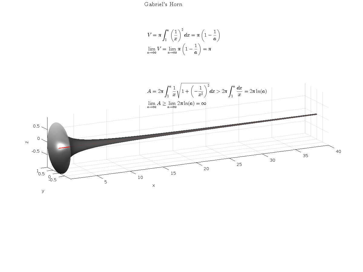
The properties of this figure were first studied by Italian physicist and mathematician Evangelista Torricelli in the 17th century.
Acknowledgment
I would like to express my sincere gratitude to all those who have supported and inspired me throughout this project.
First and foremost, I would like to thank the mathematician and my esteemed colleague, Stavros Tsalapatis, for inspiring me with the fascinating subject of Gabriel's Horn.
I am also deeply thankful to Mr. @Star Strider for his invaluable assistance in completing the final code.
References:
When it comes to MOS tube burnout, it is usually because it is not working in the SOA workspace, and there is also a case where the MOS tube is overcurrent.
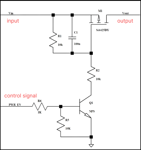
For example, the maximum allowable current of the PMOS transistor in this circuit is 50A, and the maximum current reaches 80+ at the moment when the MOS transistor is turned on, then the current is very large.
At this time, the PMOS is over-specified, and we can see on the SOA curve that it is not working in the SOA range, which will cause the PMOS to be damaged.
So what if you choose a higher current PMOS? Of course you can, but the cost will be higher.
We can choose to adjust the peripheral resistance or capacitor to make the PMOS turn on more slowly, so that the current can be lowered.
For example, when adjusting R1, R2, and the jumper capacitance between gs, when Cgs is adjusted to 1uF, The Ids are only 40A max, which is fine in terms of current, and meets the 80% derating.
(50 amps * 0.8 = 40 amps).
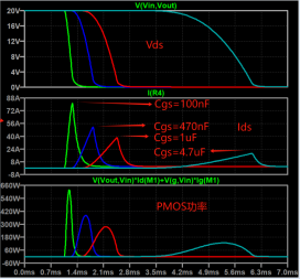
Next, let’s look at the power, from the SOA curve, the opening time of the MOS tube is about 1ms, and the maximum power at this time is 280W.
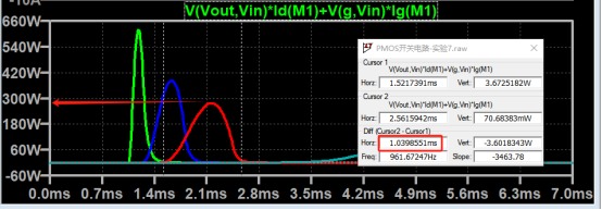
The normal thermal resistance of the chip is 50°C/W, and the maximum junction temperature can be 302°F.
Assuming the ambient temperature is 77°F, then the instantaneous power that 1ms can withstand is about 357W.
The actual power of PMOS here is 280W, which does not exceed the limit, which means that it works normally in the SOA area.
Therefore, when the current impact of the MOS transistor is large at the moment of turning, the Cgs capacitance can be adjusted appropriately to make the PMOS Working in the SOA area, you can avoid the problem of MOS corruption.
I am trying to earn my Intro to MATLAB badge in Cody, but I cannot click the Roll the Dice! problem. It simply is not letting me click it, therefore I cannot earn my badge. Does anyone know who I should contact or what to do?
I define the class in matlab as:
classdef Myclass
properties
Content
end
methods
function obj = Myclass(content)
obj.Content = content;
end
function disp(obj)
A = symmatrix('A(1/3,[0,0,1])');
disp(A);
end
end
end
When we run this class in live editor return 'A(1/3,[0,0,1])' rather than latex form.
Myclass(1)
% return 'A(1/3,[0,0,1])'
A = symmatrix('A(1/3,[0,0,1])');
% return latrx form A(1/3,[0,0,1])
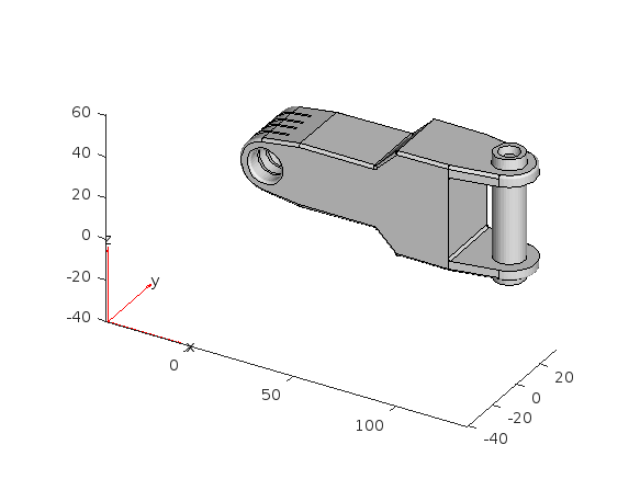
Something that had bothered me ever since I became an FEA analyst (2012) was the apparent inability of the "camera" in Matlab's 3D plot to function like the "cameras" in CAD/CAE packages.
For instance, load the ForearmLink.stl model that ships with the PDE Toolbox in Matlab and ParaView and try rotating the model.
clear
close all
gm = importGeometry( "ForearmLink.stl" );
pdegplot(gm)
Things to observe:
- Note that I cant seem to rotate continuously around the x-axis. It appears to only support rotations from [0, 360] as opposed to [-inf, inf]. So, for example, if I'm looking in the Y+ direction and rotate around X so that I'm looking at the Z- direction, and then want to look in the Y- direction, I can't simply keep rotating around the X axis... instead have to rotate 180 degrees around the Z axis and then around the X axis. I'm not aware of any data visualization applications (e.g., ParaView, VisIt, EnSight) or CAD/CAE tools with such an interaction.
- Note that at the 50 second mark, I set a view in ParaView: looking in the [X-, Y-, Z-] direction with Y+ up. Try as I might in Matlab, I'm unable to achieve that same view perspective.
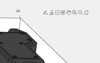
Today I discovered that if one turns on the Camera Toolbar from the View menubar, then clicks the Orbit Camera icon, then the No Principal Axis icon:
That then it acts in the manner I've long desired. Oh, and also, for the interested, it is programmatically available: https://www.mathworks.com/help/matlab/ref/cameratoolbar.html
I might humbly propose this mode either be made more discoverable, similar to the little interaction widgets that pop up in figures:
Or maybe use the middle-mouse button to temporarily use this mode (a mouse setting in, e.g., Abaqus/CAE).
Hi everyone,
I need deep orientation to make calculation of speed and Angle for the absolute encoder RM22SC with signal (data+, Data-, Clock +, Clock -) using Launchpad F28379D and Simulink.
I did interface the absolute encoder with IC DS26LS32CN and I did get signal Data and Clock. I did use the GPIO20 for Data and GPIO21 for Clock and connect both to the Matlab Function block to get as output the position. See the code on attached. The output of the Matlab function times 2*pi/8192 to get the angle. However, I don't get anything as value.
Matlab Fuction Block code
function position = decodeSSI(data, clock)
%#codegen
persistent bitCounter shiftRegister prevClock
if isempty(bitCounter)
bitCounter = uint32(0);
shiftRegister = uint32(0);
prevClock = uint32(0);
end
% Parameters
numBits = 13; % Number of bits in the SSI word
% Rising edge detection for clock
clock = uint32(clock); % Ensure clock is of type integer
clockRisingEdge = (clock == 1) && (prevClock == 0);
prevClock = clock;
if clockRisingEdge
bitCounter = bitCounter + 1;
% Shift in the data bit
shiftRegister = bitor(bitshift(shiftRegister, 1), uint32(data));
% Check if we have received the full word
if bitCounter == numBits
position = shiftRegister;
% Reset for the next word
bitCounter = uint32(0);
shiftRegister = uint32(0);
else
position = uint32(0); % or NaN to indicate incomplete data
end
else
position = uint32(0); % or retain the last valid position
end
end
I've noticed is that the highly rated fonts for coding (e.g. Fira Code, Inconsolata, etc.) seem to overlook one issue that is key for coding in Matlab. While these fonts make 0 and O, as well as the 1 and l easily distinguishable, the brackets are not. Quite often the curly bracket looks similar to the curved bracket, which can lead to mistakes when coding or reviewing code.
So I was thinking: Could Mathworks put together a team to review good programming fonts, and come up with their own custom font designed specifically and optimized for Matlab syntax?
could you explain me how to calculate the gain values for different types of controllers (Conventional Sliding Mode Control, Third Order Sliding Mode Control, Variable Gain Super Twisting Algorithm.
Could you, assist me in providing a mathematical method, for example, to calculate the gains of the above-mentioned controllers?
Thank you
M. Itouchene
Hello everyone, i hope you all are in good health. i need to ask you about the help about where i should start to get indulge in matlab. I am an electrical engineer but having experience of construction field. I am new here. Please do help me. I shall be waiting forward to hear from you. I shall be grateful to you. Need recommendations and suggestions from experienced members. Thank you.
I recently wrote up a document which addresses the solution of ordinary and partial differential equations in Matlab (with some Python examples thrown in for those who are interested). For ODEs, both initial and boundary value problems are addressed. For PDEs, it addresses parabolic and elliptic equations. The emphasis is on finite difference approaches and built-in functions are discussed when available. Theory is kept to a minimum. I also provide a discussion of strategies for checking the results, because I think many students are too quick to trust their solutions. For anyone interested, the document can be found at https://blanchard.neep.wisc.edu/SolvingDifferentialEquationsWithMatlab.pdf
hello i'm working on simulation using simulink which is my title is ENHANCING BATTERYENERGY STORAGE SYSTEMSTHROUGH MODULAR MULTILEVEL CONVERTER WITH STATE-OF-CHARGE BALANCING CONTROL. i already build 9 level mmc. but i dont have any idea for state of charge balancing control.please any suggestion and explain.
Hi,
I'm trying to write a code which can determine the gradient change in a given profile. However the code is unable to determine the same correctly and giving incorrect results. For the pic1 below it should give me the width of the region where it is a steep gradient determined.
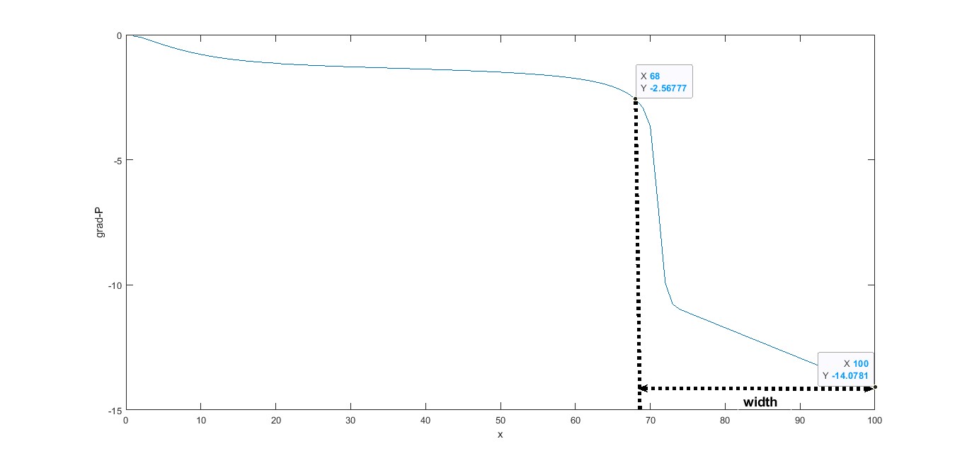
However for pic2 below it shouldn't as there is no steep gradient compared to pic1
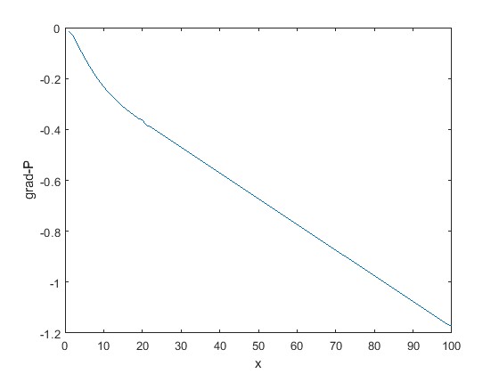
The code is as below:
clear width;
global width;
global data;
for i=1:max(length(data.variable.t))
for j=1:max(length(data.variable.x))-1
change_p = (abs(data.variable.gradpressure(i,j+1))-abs(data.variable.gradpressure(i,j)))/abs(data.variable.gradpressure(i,j));
%disp(change_p)
if change_p > 0.1
disp("steep gradient found")
width(j)=1-data.variable.x(j);
disp(width)
else
disp("no steep gradient found")
end
end
end
the data.variable.gradpressure is a 1000x100 matrix with t along the vertical and x along the horizontal.
with regards,
rc
Sub aspenaAdorption()
' Declare variables for the ACM application, document, and simulation
Dim ACMApp As Object
Dim ACMDocument As Object
Dim ACMSimulation As Object
' Create an instance of the ACM application
Set ACMApp = CreateObject("ACM Application")
' Use "ACM Application" for Aspen Custom Modeler
' Use "ADS Application" for Aspen Adsorption
' Make the ACM application visible
ACMApp.Visible = True
' Open the specified simulation document
Set ACMDocument = ACMApp.OpenDocument("C:\Users\user\Desktop\H2_Purification.acmf")
' Set the simulation object to the current simulation in the application
Set ACMSimulation = ACMApp.Simulation
' Set the simulation to run in dynamic mode
ACMSimulation.RunMode = "Dynamic"
' Run the simulation
ACMSimulation.Run (True)
' Check if the simulation was successful and display a message box
If ACMSimulation.Successful Then
MsgBox "Simulation Complete"
Else
MsgBox "Simulation Failed"
End If
' Quit the ACM application
ACMApp.Quit
End Sub