2-D Stationary Wavelet Transform

This section takes you through the features of 2-D discrete stationary wavelet analysis using the Wavelet Toolbox™ software.

Analysis-Decomposition Function

Function Name	Purpose
swt2	Decomposition

Synthesis-Reconstruction Function

Function Name	Purpose
iswt2	Reconstruction

The stationary wavelet decomposition structure is more tractable than the wavelet one. So, the utilities useful for the wavelet case are not necessary for the Stationary Wavelet Transform (SWT).

In this section, you'll learn to

• Load an image

• Analyze an image

• Perform single-level and multilevel image decompositions and reconstructions

• Denoise an image

2-D Analysis

In this example, we'll show how you can use 2-D stationary wavelet analysis to denoise an image.

Note

Instead of using image(I) to visualize the image I, we use image(wcodemat(I)), which displays a rescaled version of I leading to a clearer presentation of the details and approximations (see the wcodemat reference page).

This example involves a image containing noise.

1. Load an image.

   From the MATLAB^® prompt, type

   load noiswom 
   whos
   
   

   Name	Size	Bytes	Class
   X	96x96	73728	double array
   map	255x3	6120	double array

   For the SWT, if a decomposition at level k is needed, 2^k must divide evenly into size(X,1) and size(X,2). If your original image is not of correct size, you can use the function wextend to extend it.

2. Perform a single-level Stationary Wavelet Decomposition.

   Perform a single-level decomposition of the image using the db1 wavelet. Type

   [swa,swh,swv,swd] = swt2(X,1,'db1');
   

   This generates the coefficients matrices of the level-one approximation (swa) and horizontal, vertical and diagonal details (swh, swv, and swd, respectively). Both are of size-the-image size. Type

   whos
   
   

   Name	Size	Bytes	Class
   X	96x96	73728	double array
   map	255x3	6120	double array
   swa	96x96	73728	double array
   swh	96x96	73728	double array
   swv	96x96	73728	double array
   swd	96x96	73728	double array

3. Display the coefficients of approximation and details.

   To display the coefficients of approximation and details at level 1, type

   map = pink(size(map,1)); colormap(map) 
   subplot(2,2,1), image(wcodemat(swa,192));
   title('Approximation swa') 
   subplot(2,2,2), image(wcodemat(swh,192));
   title('Horiz. Detail swh') 
   subplot(2,2,3), image(wcodemat(swv,192));
   title('Vertical Detail swv') 
   subplot(2,2,4), image(wcodemat(swd,192));
   title('Diag. Detail swd');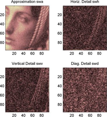
   

   

4. Regenerate the image by Inverse Stationary Wavelet Transform.

   To find the inverse transform, type

   A0 = iswt2(swa,swh,swv,swd,'db1');
   

   To check the perfect reconstruction, type

   err = max(max(abs(X-A0)))
   
   err =
        1.1369e-13
   

5. Construct and display approximation and details from the coefficients.

   To construct the level 1 approximation and details (A1, H1, V1 and D1) from the coefficients swa, swh, swv and swd, type

   nulcfs = zeros(size(swa));
   A1 = iswt2(swa,nulcfs,nulcfs,nulcfs,'db1');  
   H1 = iswt2(nulcfs,swh,nulcfs,nulcfs,'db1');
   V1 = iswt2(nulcfs,nulcfs,swv,nulcfs,'db1'); 
   D1 = iswt2(nulcfs,nulcfs,nulcfs,swd,'db1');
   

   To display the approximation and details at level 1, type

   colormap(map)
   subplot(2,2,1), image(wcodemat(A1,192)); 
   title('Approximation A1')
   subplot(2,2,2), image(wcodemat(H1,192)); 
   title('Horiz. Detail H1')
   subplot(2,2,3), image(wcodemat(V1,192)); 
   title('Vertical Detail V1')
   subplot(2,2,4), image(wcodemat(D1,192)); 
   title('Diag. Detail D1')
   

   

6. Perform a multilevel Stationary Wavelet Decomposition.

   To perform a decomposition at level 3 of the image (again using the db1 wavelet), type

   [swa,swh,swv,swd] = swt2(X,3,'db1');
   

   This generates the coefficients of the approximations at levels 1, 2, and 3 (swa) and the coefficients of the details (swh, swv and swd). Observe that the matrices swa(:,:,i), swh(:,:,i), swv(:,:,i), and swd(:,:,i) for a given level i are of size-the-image size. Type

   clear A0 A1 D1 H1 V1 err nulcfs 
   whos 
   

   Name	Size	Bytes	Class
   X	96x96	73728	double array
   map	255x3	6120	double array
   swa	96x96x3	221184	double array
   swh	96x96x3	221184	double array
   swv	96x96x3	221184	double array
   swd	96x96x3	221184	double array

7. Display the coefficients of approximations and details.

   To display the coefficients of approximations and details, type

   colormap(map)
   kp = 0; 
   for i = 1:3
       subplot(3,4,kp+1), image(wcodemat(swa(:,:,i),192));
       title(['Approx. cfs level ',num2str(i)])
       subplot(3,4,kp+2), image(wcodemat(swh(:,:,i),192));
       title(['Horiz. Det. cfs level ',num2str(i)]) 
       subplot(3,4,kp+3), image(wcodemat(swv(:,:,i),192));
       title(['Vert. Det. cfs level ',num2str(i)]) 
       subplot(3,4,kp+4), image(wcodemat(swd(:,:,i),192)); 
       title(['Diag. Det. cfs level ',num2str(i)])
       kp = kp + 4; 
   end
   

8. Reconstruct approximation at Level 3 and details from coefficients.

   To reconstruct the approximation at level 3, type

   mzero = zeros(size(swd)); 
   A = mzero; 
   A(:,:,3) = iswt2(swa,mzero,mzero,mzero,'db1');
   

   To reconstruct the details at levels 1, 2 and 3, type

   H = mzero; V = mzero; 
   D = mzero; 
   for i = 1:3
       swcfs = mzero; swcfs(:,:,i) = swh(:,:,i); 
       H(:,:,i) = iswt2(mzero,swcfs,mzero,mzero,'db1');
       swcfs = mzero; swcfs(:,:,i) = swv(:,:,i); 
       V(:,:,i) = iswt2(mzero,mzero,swcfs,mzero,'db1');
       swcfs = mzero; swcfs(:,:,i) = swd(:,:,i); 
       D(:,:,i) = iswt2(mzero,mzero,mzero,swcfs,'db1');
   end
   

9. Reconstruct and display approximations at Levels 1, 2 from approximation at Level 3 and details at Levels 1, 2, and 3.

   To reconstruct the approximations at levels 2 and 3, type

   A(:,:,2) = A(:,:,3) + H(:,:,3) + V(:,:,3) + D(:,:,3); 
   A(:,:,1) = A(:,:,2) + H(:,:,2) + V(:,:,2) + D(:,:,2);
   

   To display the approximations and details at levels 1, 2, and 3, type

   colormap(map)
   kp = 0; 
   for i = 1:3 
       subplot(3,4,kp+1), image(wcodemat(A(:,:,i),192));
       title(['Approx. level ',num2str(i)]) 
       subplot(3,4,kp+2), image(wcodemat(H(:,:,i),192));
       title(['Horiz. Det. level ',num2str(i)]) 
       subplot(3,4,kp+3), image(wcodemat(V(:,:,i),192)); 
       title(['Vert. Det. level ',num2str(i)])
       subplot(3,4,kp+4), image(wcodemat(D(:,:,i),192)); 
       title(['Diag. Det. level ',num2str(i)]) 
       kp = kp + 4; 
   end
   

10. Remove noise by thresholding.

    To denoise an image, use the ddencmp function to find the threshold value, use the wthresh function to perform the actual thresholding of the detail coefficients, and then use the iswt2 function to obtain the denoised image.

    thr = 44.5; 
    sorh = 's'; dswh = wthresh(swh,sorh,thr); 
    dswv = wthresh(swv,sorh,thr);
    dswd = wthresh(swd,sorh,thr); 
    clean = iswt2(swa,dswh,dswv,dswd,'db1');
    

    To display both the original and denoised images, type

    colormap(map)
    subplot(1,2,1), image(wcodemat(X,192)); 
    title('Original image') 
    subplot(1,2,2), image(wcodemat(clean,192)); 
    title('denoised image')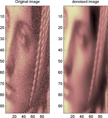
    

    

    A second syntax can be used for the swt2 and iswt2 functions, giving the same results:

    lev= 4; 
    swc = swt2(X,lev,'db1'); 
    swcden = swc; 
    swcden(:,:,1:end-1) =
    wthresh(swcden(:,:,1:end-1),sorh,thr); 
    clean = iswt2(swcden,'db1');
    

    You obtain the same plot by using the plot commands in step 9 above.