多重信号の 1 次元ウェーブレット解析

この例では次を使用します。

ライブスクリプトを開く

1 次元の多重信号は、行単位 (または列単位) で構成される行列として格納される、長さの等しい 1 次元信号のセットです。

この例では、多重信号の解析、ノイズ除去または圧縮を行い、多重信号を構成する信号のさまざまな表現または簡略化されたバージョンをクラスター化する方法を示します。

最初に、信号を解析します。次に、信号のさまざまな表現または簡略化されたバージョンを生成します。

指定のレベルで再構成した Approximation
ノイズ除去後のバージョン
圧縮後のバージョン

ノイズ除去と圧縮は、ウェーブレットの主要な用途の 2 つであり、多くの場合にクラスタリングの前の前処理手順として使用されます。

最後に、いくつかの異なるクラスタリング戦略を適用し、結果を比較します。クラスタリングを使用すると、スパースウェーブレット表現を使用して大規模な信号のセットを集計することができます。

多重信号の読み込みとプロット

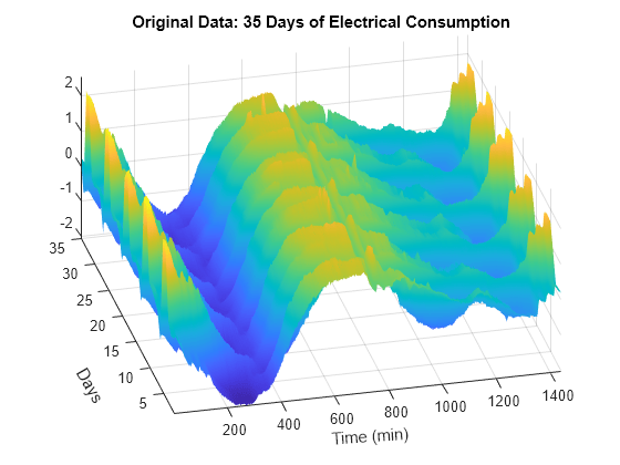
35 日間の電気負荷消費を表す多重信号を読み込み、プロットします。データは、センタリングおよび標準化されます。信号は局所的には不規則でありノイズも含んでいるが、3 種類の大まかな形状が識別できることを確認します。

load elec35_nor
X = signals;
[nbSIG,nbVAL] = size(X);
plot(X','r')
axis tight
title('Original Data: 35 Days of Electrical Consumption')
xlabel('Time (min)')

Figure contains an axes object. The axes object with title Original Data: 35 Days of Electrical Consumption, xlabel Time (min) contains 35 objects of type line.

データの表面表現

多重信号の周期性を強調するために、データの 3 次元表現を調べます。5 つの週の表現がよりはっきりと確認できます。

surf(X)
shading interp
axis tight
title('Original Data: 35 Days of Electrical Consumption')
xlabel('Time (min)','Rotation',4)
ylabel('Days','Rotation',-60)
ax = gca;
ax.View = [-13.5 48];

Figure contains an axes object. The axes object with title Original Data: 35 Days of Electrical Consumption, xlabel Time (min), ylabel Days contains an object of type surface.

多重信号の行の分解

mdwtdec を使用し、'sym4' ウェーブレットを使用して、ウェーブレット分解をレベル 7 で実行します。

dirDec = 'r';         % Direction of decomposition
level  = 7;           % Level of decomposition  
wname  = 'sym4';      % Near symmetric wavelet
decROW = mdwtdec(dirDec,X,level,wname)

decROW = struct with fields:
        dirDec: 'r'
         level: 7
         wname: 'sym4'
    dwtFilters: [1x1 struct]
       dwtEXTM: 'sym'
      dwtShift: 0
      dataSize: [35 1440]
            ca: [35x18 double]
            cd: {[35x723 double]  [35x365 double]  [35x186 double]  [35x96 double]  [35x51 double]  [35x29 double]  [35x18 double]}

レベル 7 の信号および Approximation

各行の信号のレベル 7 で Approximation を再構成します。Approximation と元の信号を比較します。レベル 7 の Approximation は全体的な形状を捉えていますが、いくつかの興味深い特徴が失われています。たとえば、信号の最初と最後のバンプが消失しています。

A7_ROW  = mdwtrec(decROW,'a',7);
subplot(2,1,1)
plot(X(:,:)','r')
title('Original Data')
axis tight 
subplot(2,1,2)
plot(A7_ROW(:,:)','b')
axis tight
title('Corresponding Approximations at Level 7')

Figure contains 2 axes objects. Axes object 1 with title Original Data contains 35 objects of type line. Axes object 2 with title Corresponding Approximations at Level 7 contains 35 objects of type line.

重ね合わされた信号および Approximation

元の信号とレベル 7 の対応する Approximation をより厳密に比較するために、最初の 4 日間の元の信号およびそれに対応する Approximation を重ねてプロットします。最後の 5 日間のデータを使用して同一のプロットを作成します。全体的な形状に関しては、元の信号の Approximation が視覚的に正確であることに注意してください。

subplot(2,1,1)
idxDays = 1:4;
plot(X(idxDays,:)','r')
hold on
plot(A7_ROW(idxDays,:)','b')
hold off
axis tight
title(['Days ' int2str(idxDays), ' - Signals and Approximations at Level 7'])
subplot(2,1,2)
idxDays = 31:35;
plot(X(idxDays,:)','r')
hold on
plot(A7_ROW(idxDays,:)','b')
hold off
axis tight
title(['Days ' int2str(idxDays), ' - Signals and Approximations at Level 7'])

Figure contains 2 axes objects. Axes object 1 with title Days 1 2 3 4 - Signals and Approximations at Level 7 contains 8 objects of type line. Axes object 2 with title Days 31 32 33 34 35 - Signals and Approximations at Level 7 contains 10 objects of type line.

多重信号のノイズ除去

明らかに電気信号に起因するこれらのバンプを維持しながら、この多重信号のより微細な単純化を実行するために、多重信号のノイズを除去します。

ノイズ除去手順は次の 3 つのステップで実行されます。

分解: ウェーブレットと分解レベル N を選択し、レベル N での信号のウェーブレット分解を取得します。
しきい値処理: 1 から N までの各レベルおよび各信号でしきい値を選択し、Detail 係数にしきい値の設定を適用します。
再構成: レベル N の元の Approximation 係数と、レベル 1 から N までの変更済みの Detail 係数を使用して、ウェーブレットの再構成を計算します。

関数 mdwtdec と関数 mswden を使用して、多重信号のノイズを除去します。前に使用した分解レベル N = 7 の代わりに、N = 5 を指定します。信号の最初と最後のバンプが十分に回復していること、それに対して残差は信号に起因する一部の残りバンプを除いてノイズのように見えることに注意してください。さらに、このような残りバンプの振幅の程度は小さいです。

dirDec = 'r';         % Direction of decomposition
level  = 5;           % Level of decomposition  
wname  = 'sym4';      % Near symmetric wavelet
decROW = mdwtdec(dirDec,X,level,wname);

[XD,decDEN] = mswden('den',decROW,'sqtwolog','mln');
Residuals = X-XD;
figure
subplot(3,1,1)
plot(X','r')
axis tight
title('Original Data: 35 Days of Electrical Consumption')
subplot(3,1,2)
plot(XD','b')
axis tight
title('Denoised Data: 35 Days of Electrical Consumption')
subplot(3,1,3)
plot(Residuals','k')
axis tight
title('Residuals')
xlabel('Time (min)')

Figure contains 3 axes objects. Axes object 1 with title Original Data: 35 Days of Electrical Consumption contains 35 objects of type line. Axes object 2 with title Denoised Data: 35 Days of Electrical Consumption contains 35 objects of type line. Axes object 3 with title Residuals, xlabel Time (min) contains 35 objects of type line.

行の信号を圧縮する多重信号

ノイズ除去のように、次の 3 つの手順を使用して圧縮手順を実行します (上記を参照)。

ノイズ除去手順との違いは、手順 2 にあります。利用可能な圧縮方法は 2 つあります。

1 番目は信号のウェーブレット拡張を利用し、最大の絶対値係数を維持します。この場合、グローバルしきい値、圧縮性能または相対的な二乗ノルムの回復性能を設定します。したがって、1 つの信号依存パラメーターのみを選択する必要があります。
2 番目のアプローチでは、決定済みのレベルに依存するしきい値を視覚的に適用します。

データ表現を簡略化し、圧縮をより効率的にするために、関数 mdwtdec と関数 mswcmp を使用します。グローバルしきい値を適用して多重信号の各行を圧縮し、エネルギーの 99% を回復させます。レベル 7 での分解を指定します。全体的な形状は維持されますが、局所的な凹凸は無視されます。残差には、基本的には小さなスケールに起因するノイズと成分が含まれています。

dirDec = 'r';         % Direction of decomposition
level  = 7;           % Level of decomposition  
wname  = 'sym4';      % Near symmetric wavelet
decROW = mdwtdec(dirDec,X,level,wname);

[XC,decCMP,THRESH] = mswcmp('cmp',decROW,'L2_perf',99);
figure
subplot(3,1,1)
plot(X','r')
axis tight
title('Original Data: 35 Days of Electrical Consumption')
subplot(3,1,2)
plot(XC','b')
axis tight
title('Compressed Data: 35 Days of Electrical Consumption')
subplot(3,1,3)
plot((X-XC)','k')
axis tight
title('Residuals')
xlabel('Time (min)')

Figure contains 3 axes objects. Axes object 1 with title Original Data: 35 Days of Electrical Consumption contains 35 objects of type line. Axes object 2 with title Compressed Data: 35 Days of Electrical Consumption contains 35 objects of type line. Axes object 3 with title Residuals, xlabel Time (min) contains 35 objects of type line.

圧縮性能

非ゼロ要素の対応する密度を計算します。各信号について、エネルギーを 99% 回復するために必要な係数の割合は 1.25% から 1.75% の間です。これは、いくつかの係数の信号エネルギーを集中させるためのウェーブレットの容量を示しています。

cfs = cat(2,[decCMP.cd{:},decCMP.ca]);
cfs = sparse(cfs);
perf = zeros(1,nbSIG);
for k = 1:nbSIG
    perf(k) = 100*nnz(cfs(k,:))/nbVAL;
end

figure
plot(perf,'r-*')
title('Percentages of Nonzero Coefficients for the 35 Days')
xlabel('Signal Indices')
ylabel('% of Nonzero Coefficients')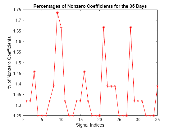

Figure contains an axes object. The axes object with title Percentages of Nonzero Coefficients for the 35 Days, xlabel Signal Indices, ylabel % of Nonzero Coefficients contains an object of type line.

行信号のクラスタリング

クラスタリングは、スパースウェーブレット表現を使用して大規模な信号のセットを集計する簡単な手続きです。関数 mdwtcluster を使用して階層クラスタリングを実装できます。mdwtcluster を使用するには、Statistics and Machine Learning Toolbox™ が必要です。

35 日間のデータの 3 つの異なるクラスタリングを比較します。1 番目は元の多重信号、2 番目はレベル 7 の Approximation 係数、最後はノイズ除去された多重信号に基づいています。

クラスター数を 3 に設定します。最初の 2 つの区画および 3 番目の区画をそれぞれ含む構造体 P1 および P2 を計算します。

P1 = mdwtcluster(decROW,'lst2clu',{'s','ca7'},'maxclust',3);
P2 = mdwtcluster(decDEN,'lst2clu',{'s'},'maxclust',3);
Clusters = [P1.IdxCLU P2.IdxCLU];

3 つの区画が同等であることを確認します。

EqualPART = isequal(max(diff(Clusters,[],2)),[0 0])

EqualPART = logical
   1

クラスターをプロットして調べます。

figure
stem(Clusters,'filled','b:')
title('The Three Clusters of the Original 35 days')
xlabel('Signal Indices')
ylabel('Index of Cluster')
ax = gca;
xlim([1 35])
ylim([0.5 3.1])
ax.YTick = 1:3;

Figure contains an axes object. The axes object with title The Three Clusters of the Original 35 days, xlabel Signal Indices, ylabel Index of Cluster contains 3 objects of type stem.

最初のクラスター (ラベル 3) には週の中頃の 25 日が含まれ、その他の 2 つ (ラベル 2 および 1) にはそれぞれ土曜日が 5 日と日曜日が 5 日含まれています。再度、これは、この例の最初に表示された最初の 2 つのプロットにみられる基底となる時系列と 3 種類の大まかな形状の周期性を示しています。

元の信号と、3 つの区画のうち 2 つを取得するために使用された対応する Approximation 係数を表示します。

CA7 = mdwtrec(decROW,'ca');
IdxInCluster = cell(1,3);
for k = 1:3
    IdxInCluster{k} = find(P2.IdxCLU==k);
end
figure('Units','normalized','Position',[0.2 0.2 0.6 0.6])
for k = 1:3
    idxK = IdxInCluster{k};
    subplot(2,3,k)
    plot(X(idxK,:)','r')
    axis tight
    ax = gca;
    ax.XTick = [200 800 1400];
    if k==2
        title('Original Signals')
    end
    xlabel(['Cluster: ' int2str(k) ' (' int2str(length(idxK)) ')'])
    subplot(2,3,k+3)
    plot(CA7(idxK,:)','b')
    axis tight
    if k==2
        title('Coefficients of Approximations at Level 7')
    end
    xlabel(['Cluster: ' int2str(k) ' (' int2str(length(idxK)) ')'])  
end

元の信号 (各信号の 1440 のサンプル) およびレベル 7 での Approximation の係数 (各信号の 18 サンプル) から同じ区画が取得されます。これは、35 日間の同じクラスタリング分割を取得するのに 2% 未満の係数の使用で十分であることを示しています。

まとめ

ウェーブレットを使用したノイズ除去、圧縮およびクラスタリングは非常に効率的な方法です。いくつかの係数の信号エネルギーを集中させるためのウェーブレット表現の能力が効率性の鍵です。さらに、クラスタリングは、スパースウェーブレット表現を使用して大規模な信号のセットを集計する簡単な手続きです。この例では、関数 mdwtdec と関数 mswden を使用して多重信号のノイズを除去しました。関数wdenoiseを使用して多重信号のノイズを除去することもできます。