Joint Time-Frequency Scattering

A joint time-frequency scattering (JTFS) network enables you to extract features from a signal that are invariant to shifts or deformations in both time and frequency. Time and frequency invariance makes JTFS features robust inputs in AI classification workflows. For more information on using JTFS in such workflows, see Acoustic Scene Classification with Wavelet Scattering and Musical Instrument Classification with Joint Time-Frequency Scattering.

Anden, Lostanlen, and Mallat developed the JTFS transform as an extension of wavelet time scattering [1]. The wavelet time scattering transform filters data along the time dimension, and then applies pointwise modulus nonlinearities. The JTFS transform additionally filters the data along the frequency dimension, followed by pointwise modulus nonlinearities.

In this example, you learn how to extend wavelet time scattering into the JTFS framework. The time wavelets are related to the separable time-frequency wavelets found in JTFS. You will visualize those wavelets and learn how they are sensitive to the time-frequency geometry of a signal. You also demonstrate the equivalence of the time lowpass filter in JTFS with the lowpass filter in wavelet time scattering.

Wavelet Time Scattering

A wavelet (time) scattering network enables you to derive low-variance features from time series data to use in AI applications. The features are insensitive to translations in time on a scale that you can specify.

In a wavelet scattering network, the input data is first convolved with wavelet filters. Then, a pointwise modulus nonlinearity is applied to the filter bank outputs. The result is the scalogram of the input data. The scalogram is then smoothed (averaged) with a lowpass (scaling) filter. The process repeats for the number of filter banks specified in the network. For more information, see Wavelet Scattering. This is a tree view of a network with two filter banks.

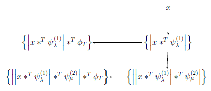
In the tree view:

• x is the input time series.

• $${\ast }^T$$ denotes convolution in time.

• $${\psi }_{\lambda }^{(1)}$$ and $${\psi }_{\mu }^{(2)}$$ are the (time) wavelets in the first- and second-order filter banks, respectively. The subscripts λ and μ correspond to the wavelet center frequencies.

• $${\phi }_T$$ is the scaling function.

By default, waveletScattering creates a scattering network with two filter banks.

The first-order scalogram coefficients

$$U_{1}x(t,\lambda )=\left|x{\ast }^T{\psi }_{\lambda }^{(1)}(t)\right|$$

are the absolute magnitude of the continuous wavelet transform (CWT) of the input data. The first-order scattering coefficients

$$S_{1}x(t,\lambda )=U_{1}x(t,\lambda ){\ast }^T{\phi }_T(t)$$

are the smoothed scalogram coefficients. The first-order scalogram and scattering coefficients are a subset of the coefficients returned by the waveletScattering object function scatteringTransform.

Joint Time-Frequency Scattering

The JTFS transform is inspired by biology. Research into the primary auditory cortex has demonstrated the existence of spectro-temporal receptive fields (STRFs) at the cortical level. The STRF of a neuron is a function of time and frequency, which describes its post-stimulus time histogram in response to various stimuli. STRFs at the cortical level exhibit ripple-like responses around a given point (t,λ) in the time-frequency domain. This ripple-like behavior can be described in terms of a temporal modulation rate, μ, and a frequency modulation rate, ℓ. The temporal modulation rate is in hertz and the frequency modulation rate is in cycles per octave or quefrency. Accordingly, the full cortical model requires four parameters: (t,λ,μ,ℓ).

The wavelets $${\psi }_{\mu }(t)=\frac{1}{\mu }\psi \left(\frac{t}{\mu }\right)$$ are used to obtain the second-order time scattering coefficients:

$$\begin{array}{ccc}{S}_{2}x(t,\lambda ,\mu )& =& \left|\left|x{\ast }^T{\psi }_{\lambda }^{(1)}\right|{\ast }^T{\psi }_{\mu }^{(2)}\right|\ast {\phi }_T(t)\\ & =& U_{2}x(t,\lambda ,\mu ){\ast }^T{\phi }_T(t).\end{array}$$

These scattering coefficients are the smoothed second-order scalogram coefficients. Both sets of coefficients are outputs of the waveletScattering object function scatteringTransform.

Joint time-frequency scattering takes wavelet time scattering one step further and creates a feature extractor that mimics the full cortical model. The second-order scattering coefficients depend on μ, the center frequencies of the second-order time wavelets, $${\psi }_{\mu }^{(2)}(t).$$ To account for the time-frequency ripple-like responses, JTFS uses a two-dimensional separable wavelet:

$${\Psi }_{\mu ,\ell ,s}(t,\lambda )={\psi }_{\mu }^{(2)}(t){\psi }_{\ell ,s}(s\lambda ).$$

The $${\psi }_{\ell ,s}(s\lambda )$$ wavelets are frequential wavelets. Recall the λ are the center frequencies of the first-order time wavelets and the superscript (2) here denotes that this wavelet is used in the second-order time scattering. The variable s is the so-called spin which takes the values ±1. Therefore, with respect to frequency modulations, the separable wavelet permits both positive and negative frequencies whereas the time wavelets are typically analytic.

Similar to the case with time scattering, in JTFS, you apply a joint time-frequency lowpass filter $${\phi }_{T,F}$$. The JTFS coefficients are defined as:

$$S(t,\lambda ,\mu ,\ell ,s)=\left|\left|x{\ast }^T{\psi }_{\lambda }^{(1)}\right|{\ast }^{T,F}{\Psi }_{\mu ,\ell ,s}\right|{\ast }^{T,F}{\phi }_{T,F}.$$

Visualize JTFS Separable 2-D Wavelet

Create a JTFS network.

jtfn = timeFrequencyScattering;

Use the filterbank object function to obtain the second-order time wavelet filter bank and its metadata.

[~,psi2f,~,timemeta] = filterbank(jtfn);
centerFrequency = timemeta{2}.xi;
minCenterFrequency = min(centerFrequency(end));
whichCF = minCenterFrequency; %#ok<*NASGU>

Use the same function to obtain the spin-up and spin-down wavelets and their metadata. The output variable frequencymeta contains the metadata for both the spin-up and spin-down wavelets.

[psifup,psifdown,~,frequencymeta] = filterbank(jtfn, ...
    FilterBank="frequency");
centerQuefrency = frequencymeta.xi;
minCenterQuefrency = min(centerQuefrency);
whichCQ = minCenterQuefrency;

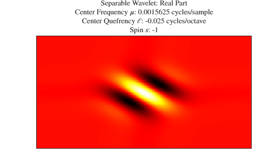
A JTFS separable 2-D wavelet $${\Psi }_{\mu ,\ell ,s}(t,\lambda )$$ is defined as ${\Psi }_{\mu ,\ell ,s}(t,\lambda )={\psi }_{\mu }^{(2)}(t){\psi }_{\ell ,s}(s\lambda )$, where $${\psi }_{\mu }^{(2)}(t)$$ is a second-order time wavelet with center frequency (time modulation rate) $$\mu$$, and $${\psi }_{\ell ,s}(s\lambda )$$ is a frequential wavelet with center quefrency (frequency modulation rate) $$\ell$$ and spin $$s$$. The frequential wavelet $${\psi }_{\ell ,1}$$ is a spin-up wavelet, and $${\psi }_{\ell ,-1}$$ is a spin-down wavelet.

Select the center frequency of a time wavelet and the center quefrency of either a spin-up or spin-down wavelet. Use the helper function helperPlotSeparableWavelet to plot the real part of the separable 2-D wavelet associated with the time and frequential wavelets. To choose a spin-down wavelet, select a negative whichCQ value. You can use the same helper function to plot the imaginary part and magnitude of $${\Psi }_{\mu ,\ell ,s}$$. The source code for this helper function is in the same folder as this example file.

whichCF = centerFrequency(9); % time wavelet center frequency
whichCQ = centerQuefrency(10); % frequential wavelet center quefrency
plotType = "real";
helperPlotSeparableWavelet(psi2f,timemeta,psifup,psifdown,frequencymeta,whichCF,whichCQ,plotType)

JTFS and Sensitivity to Time-Frequency Geometry

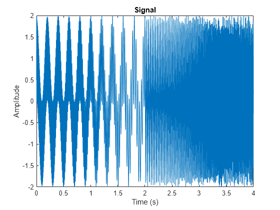
Create a signal that consists of a quadratic chirp and two sinusoids with disjoint time support. Each sinusoid has a different frequency. Sample the signal at 2000 Hz for four seconds.

tspan = 4;
Fs = 2e3;
t = 0:1/Fs:tspan-1/Fs;
y = chirp(tspan/2-t,30,max(tspan/2-t),200,"quadratic",[],"concave");
sig1 = cos(5*2*pi*t);
sig2 = cos(450*2*pi*t);
sig1 = sig1.*(t<tspan/2);
sig2 = sig2.*(t>=tspan/2);
sig = sig1+sig2+y;
plot(t,sig)
title("Signal")
xlabel("Time (s)")
ylabel("Amplitude")

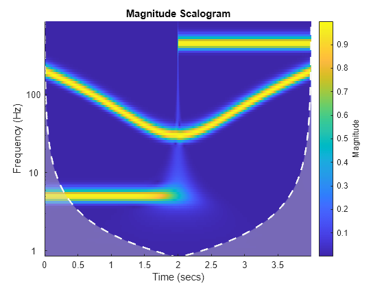
Use the cwt function to plot the scalogram of the signal. The signal has a nontrivial time-frequency geometry.

cwt(sig,Fs)

One characteristic of JTFS coefficients is that different sets of coefficients are sensitive to different parts of the time-frequency geometry. To see this, use the timeFrequencyScattering function to create a JTFS network appropriate for the signal. Use the scatteringTransform function to obtain the JTFS of the signal. The five sets of JTFS coefficients are in the dictionary outCFS, and the metadata describing each set is in the cell array outMETA.

sigLength = length(sig);
jtfn = timeFrequencyScattering(SignalLength=sigLength, ...
    TimeInvarianceScale=16, ...
    TimeQualityFactors=[16 1], ...
    TimeMaxPaddingFactor=2, ...
    FrequencyInvarianceScale=1, ...
    NumFrequencyOctaves=2, ...
    FrequencyQualityFactor=2, ...
    FrequencyMaxPaddingFactor=2);

[outCFS,outMETA] = scatteringTransform(jtfn,sig);

Use the scattergram function to visualize the spin-up and spin-down coefficients. A JTFS separable 2-D wavelet is the product of a second-order time wavelet and a frequential wavelet of spin 1 or -1. Each row in the plot corresponds to a frequential wavelet of a given center quefrency. Spin-up and spin-down wavelets have positive and negative center quefrencies, respectively. Each column corresponds to a second-order time wavelet of a given center frequency.

The spin-up coefficients preferentially localize the up-chirp portion of the quadratic chirp, and the spin-down coefficients preferentially localize the down-chirp portion. Separable wavelets with lower temporal rates and higher modulation rates tend to localize the sinusoids. Separable wavelets with higher temporal rates and lower modulation rates tend to localize the discontinuity between the sinusoids.

scattergram(jtfn,outCFS,outMETA,PlotType="Spinned")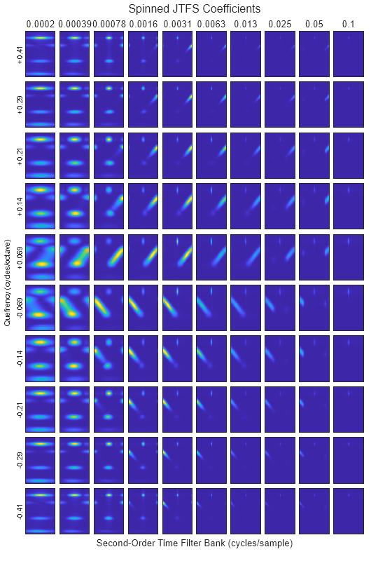

You can visualize the separable 2-D wavelet associated with a set of spinned coefficients. First, use the filterbank function to extract the second-order time wavelets and spinned wavelets from the JTFS network. Also obtain their metadata.

[~,psi2f,~,timemeta] = filterbank(jtfn);
[psifup,psifdown,~,frequencymeta] = filterbank(jtfn,FilterBank="frequency");

The variables outMETA{3} and outMETA{4} are tables describing the spin-up and spin-down coefficients, respectively. Each table row corresponds to a subplot in the scattergram, and each subplot corresponds to a specific separable 2-D wavelet. Inspect the spin-up metadata. The path table variable indicates the coefficient path. The first column is the index of the frequential wavelet, and the second column is the index of the second-order time wavelet.

outMETA{3}

ans=50×5 table
      type      log2dsfactor     path     spin    log2stride
    ________    ____________    ______    ____    __________

    "SpinUp"       0    1       1    3     1        0    4  
    "SpinUp"       0    1       2    3     1        0    4  
    "SpinUp"       0    1       3    3     1        0    4  
    "SpinUp"       0    1       4    3     1        0    4  
    "SpinUp"       0    1       5    3     1        0    4  
    "SpinUp"       0    2       1    4     1        0    4  
    "SpinUp"       0    2       2    4     1        0    4  
    "SpinUp"       0    2       3    4     1        0    4  
    "SpinUp"       0    2       4    4     1        0    4  
    "SpinUp"       0    2       5    4     1        0    4  
    "SpinUp"       0    3       1    5     1        0    4  
    "SpinUp"       0    3       2    5     1        0    4  
    "SpinUp"       0    3       3    5     1        0    4  
    "SpinUp"       0    3       4    5     1        0    4  
    "SpinUp"       0    3       5    5     1        0    4  
    "SpinUp"       0    4       1    6     1        0    4  
      ⋮

You can use the path variable to access in timemeta and frequencymeta the metadata that describes the time and frequential wavelets. Choose a path value from one of the rows in outMETA{3}. Use that value to display the metadata describing the frequential and second-order time wavelets associated with the separable wavelet. The xi variable contains the center quefrency and center frequency of the frequential and time wavelets, respectively. Metadata describing the second-order time filter bank is in timemeta{2}.

pathValue = [3 10];
frequencymeta(pathValue(1),:)

ans=1×7 table
      xi        sigma      isCQT    log2dsfactor    spin    peakidx     bwidx  
    _______    ________    _____    ____________    ____    _______    ________

    0.20711    0.042681      1           0           1        32       14    49

timemeta{2}(pathValue(2),:)

ans=1×6 table
        xi          sigma       isCQT    log2dsfactor    peakidx     bwidx 
    __________    __________    _____    ____________    _______    _______

    0.00078125    0.00031279      1           8            13       2    25

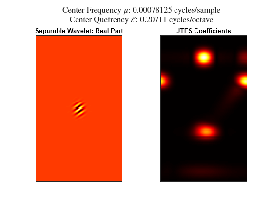
Use the helper function helperPlotJTFSWaveletAndCFS to plot the separable wavelet and the coefficients associated with it. The source code for this helper function is in the same folder as this example file.

figure
plotType = "real";
helperPlotJTFSWaveletAndCFS(pathValue,psifup,frequencymeta,psi2f,timemeta,outCFS{"SpinUp"},outMETA{3},plotType)

Equivalence of JTFS and Wavelet Time Scattering Lowpass Filters

Joint time-frequency scattering is an extension of wavelet time scattering. This example shows the equivalence of the time lowpass filter in a JTFS network with the lowpass filter in a wavelet time scattering network.

Create a wavelet time scattering network. Specify a signal length of $$2^{16}$$ samples and single precision. If the signal intended for the network is sampled at 10 kHz, then one second of data corresponds to 10,000 samples. Set the invariance scale to 10,000 samples.

slen = 2^16;
invscale = 1e4;
tsn = waveletScattering(SignalLength=slen, ...
    Precision="single", ...
    InvarianceScale=invscale);

Use the time scattering filterbank object function to obtain the lowpass (scaling) filter.

tsnfb = filterbank(tsn);
phifTS = tsnfb{1}.phift;

The time invariance scale determines the size of the time support of the lowpass filter. The scalogram coefficients are smoothed with a lowpass filter to obtain the scattering coefficients. So the time invariance scale determines how much smoothing in time is done.

To show the equivalence of the two lowpass filters, you need to determine the relationship between the time invariance scale in waveletScattering and the time invariance scale in timeFrequencyScattering. A literature search shows there is no single definition for the time invariance scale. In this example, for a given time invariance scale in wavelet time scattering, you learn how to determine the corresponding time invariance scale in JTFS. In other words, you learn how to perform equivalent smoothing, in time, in wavelet time scattering and JTFS.

To begin, for the normal distribution, 99.5% of the probability is localized in the interval $$[-2.5758{\sigma }_t,2.5758{\sigma }_t]$$, where $${\sigma }_t$$ is the time standard deviation. In wavelet time scattering, which uses the Gaussian lowpass filter $$\varphi (t)=\frac{1}{\sqrt{2\pi {\sigma }_t^2}}\exp \left(\frac{-t^2}{2{\sigma }_t^2}\right)$$, the invariance scale $$T$$ corresponds to $$\pm 2.5758{\sigma }_t$$, that is, $$T=(2\cdot 2.5758){\sigma }_t$$. You can rewrite the equation to express the time standard deviation in terms of the invariance scale: $${\sigma }_t=\frac{T}{2\cdot 2.5758}$$.

In JTFS, consider the Gaussian lowpass filter $$\varphi (t)$$ as expressed in the Fourier domain: $$\underset{}{\overset{ˆ}{\varphi }}(\xi )=\exp \left(\frac{-{\xi }^2}{2{\sigma }_{\xi }^2}\right)$$, where $${\sigma }_{\xi }^2=\frac{1}{4{\pi }^2{\sigma }_t^2}$$ which simplifies to $${\sigma }_{\xi }=\frac{1}{2\pi {\sigma }_t}$$. The presence of the '$$2\pi$$' is because JTFS uses cyclic frequency. $$\underset{}{\overset{ˆ}{\varphi }}(\xi )$$ is constructed on the frequency grid $$(-1/2,1/2)$$. Because the JTFS invariance scale $$\tau$$ is greater than or equal to 1, JTFS defines the frequency standard deviation as $${\sigma }_{\xi }=0.13/\tau$$. For the purposes of this example, $$0.13$$ is called the base sigma. Suppose $$\tau =1$$. Then $$\underset{}{\overset{ˆ}{\varphi }}(\xi )=\exp \left(\frac{-{\xi }^2}{2\cdot {(0.13)}^2}\right)$$. Because $$1/0.13$$ is approximately $$7.69$$, this means that the interval $$(-1/2,1/2)$$ contains almost 8 standard deviations, ensuring that $$\underset{}{\overset{ˆ}{\varphi }}(\xi )$$ is completely decayed. You can choose a smaller base sigma, but there would be negligible practical benefit. Note that as $$\tau$$ gets larger, the number of standard deviations in the interval grows, meaning the tails go to 0 faster. The Gaussian filter becomes more narrow in the Fourier domain, or equivalently, more broad in the time domain. Because $${\sigma }_{\xi }=\frac{1}{2\pi {\sigma }_t}$$ and $${\sigma }_{\xi }=0.13/\tau$$, you can express the time standard deviation in terms of the JTFS invariance scale: $${\sigma }_t=\frac{1}{2\pi {\sigma }_{\xi }}=\frac{1}{2\pi \cdot \left(\frac{0.13}{\tau }\right)}=\frac{\tau }{2\pi \cdot 0.13}$$.

So there are two equivalent expressions for the time standard deviation:

• Time Scattering: $${\sigma }_t^{\text{(TS)}}=\frac{T}{2\cdot 2.5758}$$

• JTFS: $${\sigma }_t^{\text{(JTFS)}}=\frac{\tau }{2\pi \cdot 0.13}$$

By equating the two expressions:

$$\frac{T}{2\cdot 2.5758}=\frac{\tau }{2\pi \cdot 0.13}$$

you can determine the JTFS invariance scale $$\tau$$ that is equivalent to a given time-scattering invariance scale $$T$$: $$\tau =\frac{2\pi \cdot 0.13}{2\cdot 2.5758}T$$.

In the time scattering network, the invariance scale $$T$$ is 10,000 samples. Determine the equivalent time invariance scale $$\tau$$ in JTFS. Round the result to obtain an integer.

basesigma = 0.13;
tau = round((2*pi*basesigma)/(2*2.5758)*invscale)

tau = 
1586

Create a JTFS network with a signal length of $$2^{16}$$. Set the time invariance scale to tau . Specify single precision and a base-2 time maximum padding factor of 0. (For more information about the padding factor, see filterpadding.) Use the JTFS filterbank object function to obtain the time lowpass filter.

jtfsn = timeFrequencyScattering(SignalLength=slen, ...
    TimeInvarianceScale=tau, ...
    FilterDataType="single", ...
    TimeMaxPaddingFactor=0);
[~,~,phifJTFS] = filterbank(jtfsn);

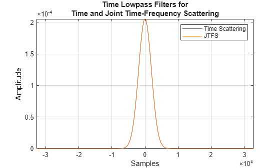
Plot both lowpass filters in the time domain. Confirm the filters are equivalent.

phitTS = ifftshift(ifft(phifTS));
phitJTFS = ifftshift(ifft(phifJTFS));
t = -slen/2:slen/2-1;
plot(t,[phitTS phitJTFS]);
grid on
axis tight
xlabel("Samples")
ylabel("Amplitude")
title(["Time Lowpass Filters for"; ...
    "Time and Joint Time-Frequency Scattering"])
legend("Time Scattering","JTFS")

References

[1] Andén, Joakim, Vincent Lostanlen, and Stéphane Mallat. “Joint Time–Frequency Scattering.” IEEE Transactions on Signal Processing 67, no. 14 (July 15, 2019): 3704–18. https://doi.org/10.1109/TSP.2019.2918992

[2] Lostanlen, Vincent, Christian El-Hajj, Mathias Rossignol, Grégoire Lafay, Joakim Andén, and Mathieu Lagrange. “Time–Frequency Scattering Accurately Models Auditory Similarities between Instrumental Playing Techniques.” EURASIP Journal on Audio, Speech, and Music Processing 2021, no. 1 (December 2021): 3. https://doi.org/10.1186/s13636-020-00187-z

[3] Mallat, Stéphane. “Group Invariant Scattering.” Communications on Pure and Applied Mathematics 65, no. 10 (October 2012): 1331–98. https://doi.org/10.1002/cpa.21413