Human Health Monitoring Using Continuous Wave Radar and Deep Learning
This example shows how to reconstruct electrocardiogram (ECG) signals via continuous wave (CW) radar signals using deep learning neural networks.
Radar is now being used for vital sign monitoring. This method offers many advantages over wearable devices. It allows non-contact measurement which is preferred for use in cases of daily use of long-term monitoring. However, the challenge is that we need to convert radar signals to vital signs or to meaningful biosignals that can be interpreted by physicians. Current traditional methods based on signal transform and correlation analysis can capture periodic heartbeats but fail to reconstruct the ECG signal from the radar returns. This example shows how AI, specifically a deep learning network, can be used to reconstruct ECG signals solely from the radar measurements.
This example uses a hybrid convolutional autoencoder and bidirectional long short-term memory (BiLSTM) network as the model. Then, a wavelet multiresolution decomposition layer, maximal overlap discrete wavelet transform (MODWT) layer, is introduced to improve the performance. The example compares the network using a 1-D convolutional layer and network using a MODWT layer.
Data Description
The dataset [1] presented in this example consists of synchronized data from a CW radar and ECG signals measured simultaneously by a reference device on 30 healthy subjects. The implemented CW radar system is based on the Six-Port technology and operates at 24 GHz in the Industrial Scientific and Medical (ISM) band.
Due to the large volume of the original dataset, for efficiency of model training, only a small subset of the data is used in this example. Specifically, the data from three scenarios, resting, apnea, and Valsalva maneuver, is selected. Further, the data from subjects 1-5 is used to train and validate the model. The data from subject 6 is used to test the trained model.
Also, because the main information contained in the ECG signal is usually located in a frequency band less than 100 Hz, all signals are downsampled to 200 Hz and divided into segments of 1024 points, i.e. signals of approximately 5s.
Download and Prepare Data
The data has been uploaded to this location: https://ssd.mathworks.com/supportfiles/SPT/data/SynchronizedRadarECGData.zip.
Download the dataset using the downloadSupportFile function. The whole dataset is approximately 16 MB in size. It contains two folders, trainVal for training and validation data and test for test data. Inside each of them, ECG signals and radar signals are stored in two separate folders, ecg and radar.
datasetZipFile = matlab.internal.examples.downloadSupportFile('SPT','data/SynchronizedRadarECGData.zip');
datasetFolder = fullfile(fileparts(datasetZipFile),'SynchronizedRadarECGData');
if ~exist(datasetFolder,'dir')
    unzip(datasetZipFile,datasetFolder);
end
Create signal datastores to access the data in the files.
radarTrainValDs = signalDatastore(fullfile(datasetFolder,"trainVal","radar"));
radarTestDs = signalDatastore(fullfile(datasetFolder,"test","radar"));
ecgTrainValDs = signalDatastore(fullfile(datasetFolder,"trainVal","ecg"));
ecgTestDs = signalDatastore(fullfile(datasetFolder,"test","ecg"));
View the categories and distribution of the data contained in the training and test sets. Note the GDN000X represents measurement data from subject X and not every subject has data for all three scenarios.
trainCats = filenames2labels(radarTrainValDs,'ExtractBefore','_radar');
summary(trainCats)
     GDN0001_Resting        59
     GDN0001_Valsalva       97
     GDN0002_Resting        60
     GDN0002_Valsalva       97
     GDN0003_Resting        58
     GDN0003_Valsalva      103
     GDN0004_Apnea          14
     GDN0004_Resting        58
     GDN0004_Valsalva      106
     GDN0005_Apnea          14
     GDN0005_Resting        59
     GDN0005_Valsalva      105
testCats = filenames2labels(radarTestDs,'ExtractBefore','_radar');
summary(testCats)
     GDN0006_Apnea          14
     GDN0006_Resting        59
     GDN0006_Valsalva      127
Apply normalization on ECG signals. Center each signal by subtracting its median and rescale it so that its maximum peak is 1.
ecgTrainValDs = transform(ecgTrainValDs,@helperNormalize);
ecgTestDs = transform(ecgTestDs,@helperNormalize);
Combine radar and ECG signal datastores. Then, further split the training and validation dataset. Use 90% of data for training and 10% for validation. Set the random seed so that data segmentation and visualization results are reproducible.
trainValDs = combine(radarTrainValDs,ecgTrainValDs);
testDs = combine(radarTestDs,ecgTestDs);

rng("default")
splitIndices = splitlabels(trainCats,0.85);
numTrain = length(splitIndices{1})
numTrain = 704
numVal = length(splitIndices{2})numVal = 126
numTest = length(testCats)
numTest = 200
trainDs = subset(trainValDs,splitIndices{1});
valDs = subset(trainValDs,splitIndices{2});
Because the dataset used here is not large, read the training, testing, and validation data into memory.
trainData = readall(trainDs);
valData = readall(valDs);
testData = readall(testDs);
Preview Data
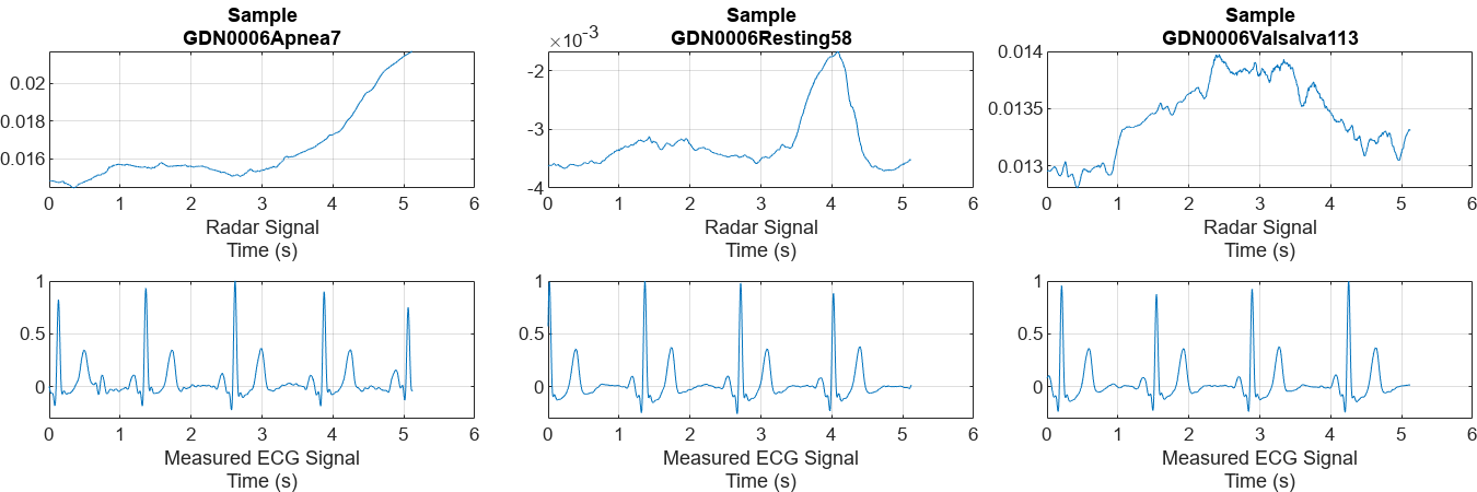
Plot a representative of each type of signal. Notice that it is almost impossible to identify any correlation between the radar signals and the corresponding reference ECG measurements.
numCats = cumsum(countcats(testCats));
previewindices = [randi([1,numCats(1)]),randi([numCats(1)+1,numCats(2)]),randi([numCats(2)+1,numCats(3)])];
testindices = [randi([1,numCats(1)]),randi([numCats(1)+1,numCats(2)]),randi([numCats(2)+1,numCats(3)])];

helperPlotData(testDs,previewindices);
Train Convolutional Autoencoder and BiLSTM Model
Build a hybrid convolutional autoencoder and BiLSTM network to reconstruct ECG signals. The first 1-D convolutional layer filters the signal. Then, the convolutional autoencoder eliminates most of the high-frequency noise and captures the high-level patterns of the whole signal. The subsequent BiLSTM layer further finely shapes the signal details.
layers1 = [
    sequenceInputLayer(1,MinLength = 1024)

    convolution1dLayer(4,3,Padding="same")
    layerNormalizationLayer()
    dropoutLayer(0.2)

    convolution1dLayer(64,8,Padding="same",Stride=8)
    reluLayer
    batchNormalizationLayer
    dropoutLayer(0.2)

    maxPooling1dLayer(2,Padding="same")

    convolution1dLayer(32,8,Padding="same",Stride=4)
    reluLayer
    batchNormalizationLayer

    maxPooling1dLayer(2,Padding="same")

    transposedConv1dLayer(32,8,Cropping="same",Stride=4)
    reluLayer

    transposedConv1dLayer(64,8,Cropping="same",Stride=8)

    bilstmLayer(8)

    fullyConnectedLayer(4)

    fullyConnectedLayer(2)

    fullyConnectedLayer(1)
];
Define the training option parameters: use an Adam optimizer and choose to shuffle the data at every epoch. Also, specify radarVal and ecgVal as the source for the validation data. Use the trainnet function to train the model. At the same time, the training information is recorded, which will be used for performance analysis and comparison later.
Train on a GPU if one is available. Using a GPU requires Parallel Computing Toolbox™ and a supported GPU device. For information on supported devices, see GPU Computing Requirements (Parallel Computing Toolbox) (Parallel Computing Toolbox).
options = trainingOptions("adam",...
    MaxEpochs=800,...
    MiniBatchSize=900,...
    InitialLearnRate=0.001,...
    ValidationData={valData(:,1),valData(:,2)},...
    ValidationFrequency=40,...
    VerboseFrequency=40,...
    Verbose=1, ...
    Shuffle="every-epoch",...
    OutputNetwork="best-validation", ...
    Plots="none", ...
    InputDataFormats="CTB", ...
    TargetDataFormats="CTB");

lossFcn = @(y,t)sum(mse(y,t),3);
[net1,info1] = trainnet(trainData(:,1),trainData(:,2),layers1,lossFcn,options);
    Iteration    Epoch    TimeElapsed    LearnRate    TrainingLoss    ValidationLoss
    _________    _____    ___________    _________    ____________    ______________
            0        0       00:00:10        0.001                            18.144
            1        1       00:00:12        0.001          18.339
           40       40       00:00:40        0.001          16.962            16.836
           80       80       00:00:57        0.001          16.955            16.868
          120      120       00:01:14        0.001          16.951            16.861
          160      160       00:01:36        0.001           16.95            16.864
          200      200       00:01:58        0.001          16.946             16.88
          240      240       00:02:17        0.001          16.942            16.908
          280      280       00:02:35        0.001          16.932            16.882
          320      320       00:02:50        0.001          16.908             16.89
          360      360       00:03:10        0.001          16.828            16.751
          400      400       00:03:25        0.001          16.718             16.86
          440      440       00:03:40        0.001          16.916            16.814
          480      480       00:03:57        0.001          16.888            16.783
          520      520       00:04:21        0.001          16.872            16.747
          560      560       00:04:35        0.001          16.764             16.62
          600      600       00:04:50        0.001          16.496            16.222
          640      640       00:05:05        0.001          16.349            15.959
          680      680       00:05:19        0.001          16.334              15.9
          720      720       00:05:35        0.001           16.22            15.912
          760      760       00:05:50        0.001          16.237            15.921
          800      800       00:06:05        0.001          16.174            15.768
Training stopped: Max epochs completed
Analyze Performance of Trained Model
Randomly pick a representative sample of each type from the test dataset to visualize and get an initial intuition about the accuracy of the reconstructions of the trained model.
helperPlotData(testDs,testindices,net1);
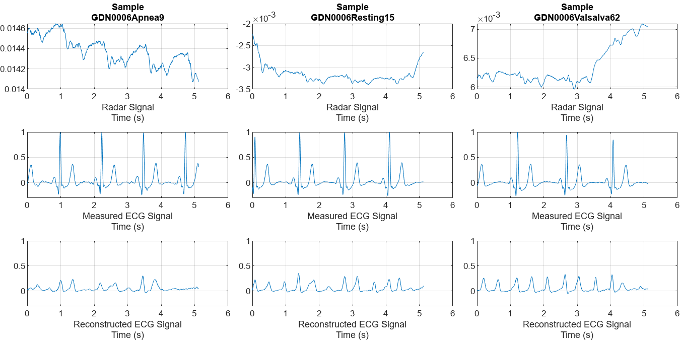
Comparing the measured and reconstructed ECG signals, it can be seen that the model has been able to initially learn some correlations between the radar and ECG signals. But the results are not very satisfactory. Some peaks are not aligned with the actual peaks and the waveform shapes do not resemble those of the measured ECG. A few peaks are even completely lost.
Improve Performance Using Multiresolution Analysis and MODWT Layer
Feature extraction is often used to capture the key information of the signals, reduce the dimensionality and redundancy of the data, and help the model achieve better results. Considering that the effective information of the ECG signal exists in a certain frequency range. Use MODWT to decompose the radar signals and get the multiresolution analysis (MRA) of it as the feature.
It can be found that some components of the radar signal decomposed by MODWTMRA, such as the component of level 4, have similar periodic patterns with the measured ECG signal. Meanwhile, some components contain almost complete noise. Inspired by this, introducing MODWT layer into the model and selecting only a few level components may help the network focus more on correlated information, while also reducing irrelevant interference.
ds = subset(trainDs,1);
[~,name,~] = fileparts(ds.UnderlyingDatastores{1}.Files{1});
data = read(ds);
radar = data{1};
ecg = data{2};

levs = 1:6;
idx = 100:800;
m = modwt(radar,'sym4',max(levs));
nplot = length(levs)+2;
mra = modwtmra(m);

figure
tiledlayout(nplot,1)
nexttile
plot(ecg(idx))
title(["ECG Signal and Radar Signal MODWTMRA", "of Sample " + regexprep(name, {'_','radar'}, '')])
ylabel("Measured ECG")
grid on
d = 1;
for i = levs
    d = d+1;
    nexttile
    plot(mra(i,idx))
    ylabel(["Radar", "MODWTMRA", "Level " + i'])
    grid on
end
nexttile
plot(mra(i+1,idx))
ylabel(["Radar", "MODWTMRA","Scaling","Coefficients"])
grid on
set(gcf,'Position',[0 0 700,800])
Replace the first convolution1dLayer with modwtLayer. The MODWT layer has been configured to have the same filter size and number of output channels to preserve the number of learning parameters. Based on the observations before, only components of a specific frequency range are preserved, i.e. level 3 to 5, which effectively removes unnecessary signal information that is irrelevant to the ECG reconstruction. Refer to modwtLayer documentation for more details on modwtLayer and these parameters.
A flattenLayer is also inserted after the modwtLayer to make the subsequent convolution1dLayer convolve along the time dimension, and to make the output format compatible with the subsequent bilstmLayer.
layers2 = [
    sequenceInputLayer(1,MinLength = 1024)

    modwtLayer('Level',5,'IncludeLowpass',false,'SelectedLevels',3:5,"Wavelet","sym4")
    flattenLayer
    layerNormalizationLayer()
    dropoutLayer(0.2)

    convolution1dLayer(64,8,Padding="same",Stride=8)
    reluLayer
    batchNormalizationLayer
    dropoutLayer(0.2)

    maxPooling1dLayer(2,Padding="same")

    convolution1dLayer(32,8,Padding="same",Stride=4)
    reluLayer
    batchNormalizationLayer

    maxPooling1dLayer(2,Padding="same")

    transposedConv1dLayer(32,8,Cropping="same",Stride=4)
    reluLayer

    transposedConv1dLayer(64,8,Cropping="same",Stride=8)

    bilstmLayer(8)

    fullyConnectedLayer(4)

    fullyConnectedLayer(2)

    fullyConnectedLayer(1)
    ];
Use the same training options as before.
options = trainingOptions("adam",...
    MaxEpochs=800,...
    MiniBatchSize=900,...
    InitialLearnRate=0.001,...
    ValidationData={valData(:,1),valData(:,2)},...
    ValidationFrequency=40,...
    VerboseFrequency=40,...
    Verbose=1, ...
    Shuffle="every-epoch",...
    OutputNetwork="best-validation", ...
    Plots="none", ...
    InputDataFormats="CTB", ...
    TargetDataFormats="CTB");

lossFcn = @(y,t)sum(mse(y,t),3);
[net2,info2] = trainnet(trainData(:,1),trainData(:,2),layers2,lossFcn,options);
    Iteration    Epoch    TimeElapsed    LearnRate    TrainingLoss    ValidationLoss
    _________    _____    ___________    _________    ____________    ______________
            0        0       00:00:08        0.001                            18.136
            1        1       00:00:09        0.001          19.273
           40       40       00:00:36        0.001          16.703            16.764
           80       80       00:01:00        0.001          14.321            14.273
          120      120       00:01:23        0.001          11.335            10.619
          160      160       00:01:45        0.001          9.5305            8.3391
          200      200       00:02:14        0.001          8.5322            7.6323
          240      240       00:02:46        0.001           7.911            7.2792
          280      280       00:03:09        0.001          7.5802            7.0774
          320      320       00:03:30        0.001          7.3912            6.9763
          360      360       00:03:53        0.001          7.1857            6.8751
          400      400       00:04:14        0.001          6.9099            6.7819
          440      440       00:04:35        0.001          6.7748            6.9208
          480      480       00:04:55        0.001          6.6766            6.8344
          520      520       00:05:25        0.001          6.4978            6.6761
          560      560       00:05:46        0.001           6.442             6.734
          600      600       00:06:06        0.001          6.3567            6.7029
          640      640       00:06:26        0.001          6.2753            6.7114
          680      680       00:06:47        0.001          6.2243            6.7499
          720      720       00:07:08        0.001          6.0981            6.6829
          760      760       00:07:29        0.001           5.999            6.6683
          800      800       00:07:50        0.001          6.0931            6.6166
Training stopped: Max epochs completed
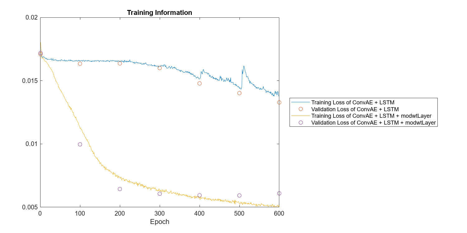
Compare the training and validation losses of two models. Both the training loss and validation loss of the model with MODWT layer drop much faster and more smoothly.
figure
plot(info1.TrainingHistory,"Iteration","Loss")
hold on
scatter(info1.ValidationHistory,"Iteration","Loss")
plot(info2.TrainingHistory,"Iteration","Loss")
scatter(info2.ValidationHistory,"Iteration","Loss")
hold off
legend(["Training Loss of ConvAE + LSTM", ...
    "Validation Loss of ConvAE + LSTM", ...
    "Training Loss of ConvAE + LSTM + modwtLayer",...
    "Validation Loss of ConvAE + LSTM + modwtLayer"],"Location","eastoutside")
xlabel("Epoch")
grid on
title("Training Information")
set(gcf,'Position',[0 0 1000,500]);
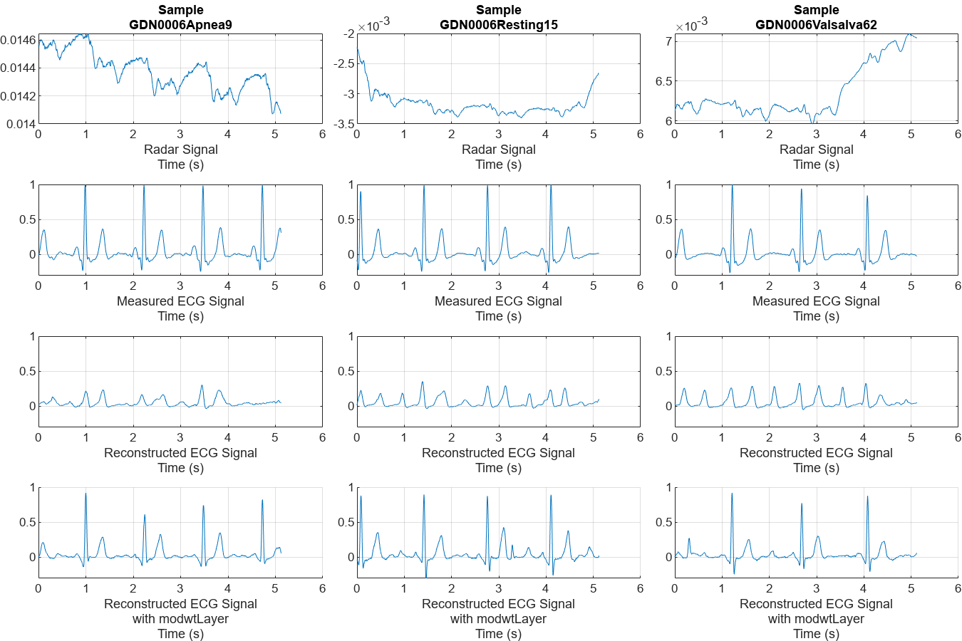
Further compare the reconstructed signals on the same test data samples. The model with modwtLayer can capture the peak position, magnitude, and shape of ECG signals very well in resting and valsalva scenarios. Even in apnea scenarios, with relatively few training samples, it can still capture the main peaks and get reconstructed signals.
helperPlotData(testDs,testindices,net1,net2)
Compare the distributions of the reconstructed signal errors for the two models on the full test set. It further illustrates that using MODWT layer improves the accuracy of the reconstruction.
ecgTestRe1 = minibatchpredict(net1,testData(:,1),InputDataFormats="CTB");
ecgTestReCell1 = squeeze(mat2cell(ecgTestRe1,1,1024,ones(200,1)));
loss1 = cellfun(@mse,ecgTestReCell1,testData(:,2));
ecgTestRe2 = minibatchpredict(net2,testData(:,1),InputDataFormats="CTB");
ecgTestReCell2 = squeeze(mat2cell(ecgTestRe2,1,1024,ones(200,1)));
loss2 = cellfun(@mse,ecgTestReCell2,testData(:,2));

figure
h1 = histogram(loss1);
hold on
h2 = histogram(loss2);
hold off

h1.Normalization = 'probability';
h1.BinWidth = 0.003;
h2.Normalization = 'probability';
h2.BinWidth = 0.003;
ylabel("Probability")
xlabel("MSE between Measured and Reconstructed ECG Signals")
title("Distribution of Test MSEs")
legend(["Model without modwtLayer","Model with modwtLayer"])

Conclusion
This example implements a convolutional autoencoder and BiLSTM network to reconstruct ECG signals from CW radar signals. The example analyzes the performance of the model with and without a MODWT Layer. It shows that the introduction of MODWT layer improves the quality of the reconstructed ECG signals.
Reference
[1] Schellenberger, S., Shi, K., Steigleder, T. et al. A dataset of clinically recorded radar vital signs with synchronized reference sensor signals. Sci Data 7, 291 (2020). https://doi.org/10.1038/s41597-020-00629-5
Appendix — Helper Functions
helperNormalize - this function normalizes input signals by subtracting the median and dividing by the maximum value.
function x = helperNormalize(x)
% This function is only intended to support this example. It may be changed
% or removed in a future release.
    x = x-median(x);
    x = {x/max(x)};
end
helperPlotData - this function plots radar and ECG signals.
function  helperPlotData(DS,Indices,net1,net2)
% This function is only intended to support this example. It may be changed
% or removed in a future release.
    arguments
       DS
       Indices
       net1 =[]
       net2 = []
    end
    fs = 200;
    N = numel(Indices);
    M = 2;
    if ~isempty(net1)
        M = M + 1;
    end
    if ~isempty(net2)
        M = M + 1;
    end

    tiledlayout(M, N, 'Padding', 'none', 'TileSpacing', 'compact');
    for i = 1:N
        idx = Indices(i);
        ds = subset(DS,idx);
        [~,name,~] = fileparts(ds.UnderlyingDatastores{1}.Files{1});
        data = read(ds);
        radar = data{1};
        ecg = data{2};
        t = linspace(0,length(radar)/fs,length(radar));

        nexttile(i)
        plot(t,radar)
        title(["Sample",regexprep(name, {'_','radar'}, '')])
        xlabel(["Radar Signal","Time (s)"])
        grid on

        nexttile(N+i)
        plot(t,ecg)
        xlabel(["Measured ECG Signal","Time (s)"])
        ylim([-0.3,1])
        grid on

        if ~isempty(net1)
            nexttile(2*N+i)
            y = minibatchpredict(net1,radar,InputDataFormats="CTB");
            plot(t,y)
            grid on
            ylim([-0.3,1])
            xlabel(["Reconstructed ECG Signal","Time (s)"])
        end

        if ~isempty(net2)
            nexttile(3*N+i)
            y = minibatchpredict(net2,radar,InputDataFormats="CTB");
            hold on
            plot(t,y)
            hold off
            grid on
            ylim([-0.3,1])
            xlabel(["Reconstructed ECG Signal", "with modwtLayer","Time (s)"])
        end

    end
    set(gcf,'Position',[0 0 300*N,150*M])
end