wmpalg
(Not recommended) Matching pursuit
The wmpalg function no longer supports plotting and is no longer
recommended. See Version History.
Syntax
Description
Examples
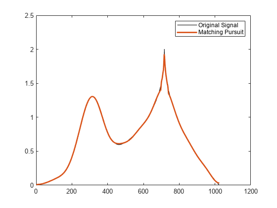
Approximate the cuspamax signal with the dictionary using orthogonal matching pursuit.
Use a dictionary consisting of sym4 wavelet packets and the DCT-II basis.
load cuspamax
yfit = wmpalg('OMP',cuspamax,'lstcpt',{{'wpsym4',2},'dct'});
plot(cuspamax,'k')
hold on
plot(yfit,'linewidth',2)
hold off
legend('Original Signal','Matching Pursuit')
Obtain the expansion coefficients in the dictionary, the column indices of the selected dictionary atoms, and the proportion of retained signal energy.
Specify a dictionary consisting of sym4 wavelet packets and the DCT-II basis. Approximate the cuspamax signal with the dictionary using orthogonal matching pursuit.
load cuspamax;
[yfit,r,coeff,iopt,qual] = wmpalg('OMP',cuspamax,...
    'lstcpt',{{'wpsym4',2},'dct'});
This example shows how to set the maximum number of iterations of the orthogonal matching pursuit to 50.
load cuspamax
[yfit,r,coeff,iopt,qual] = wmpalg('OMP',cuspamax,...
    'lstcpt',{{'wpsym4',1},{'wpsym4',2},'dct'},...
    'itermax',50);
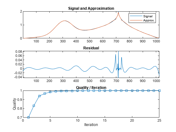
This example shows how to allow for a suboptimal choice in the update of the orthogonal matching pursuit.
Load a signal.
load cuspamaxApproximate the signal using weak orthogonal matching pursuit. Relax the requirement to be 0.8 times the optimal assignment.
[yfit,r,coeff,iopt,qual] = wmpalg('WMP',cuspamax,...
    'lstcpt',{{'wpsym4',1},{'wpsym4',2},'dct'},...
    'wmpcfs',0.8);
Plot the signal, approximation, residual, and the proportion of retained signal energy for each iteration in the matching pursuit result.
subplot(3,1,1)
plot(cuspamax)
hold on
plot(yfit)
hold off
legend('Signal','Approx.')
title('Signal and Approximation')
axis tight
subplot(3,1,2)
plot(r)
title('Residual')
axis tight
subplot(3,1,3)
plot(qual,'s-')
title('Quality / Iteration')
ylabel('Quality')
xlabel('Iteration')
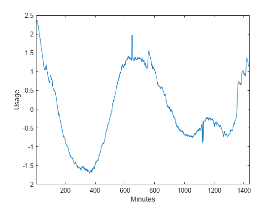
Obtain a matching pursuit of electricity consumption measured every minute over a 24-hour period.
Load and plot data. The data shows electricity consumption sampled every minute over a 24-hour period. Because the data is centered, the actual usage values are not interpretable.
load elec35_nor
y = signals(32,:);
plot(y)
xlabel("Minutes")
ylabel("Usage")
xlim([1 1440])
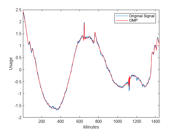
Specify a dictionary for matching pursuit consisting of the Daubechies' extremal-phase wavelet with 2 vanishing moments at level 2, the Daubechies' least-asymmetric wavelet with 4 vanishing moments at levels 1 and 4, the discrete cosine transform-II basis, and the sine basis.
dictionary = {{'db4',2},'dct','sin',{'sym4',1},{'sym4',4}};Implement orthogonal matching pursuit to obtain a signal approximation in the dictionary. Use 35 iterations. Plot the result.
[yfit,r,coef,iopt,qual] = wmpalg("OMP",y, ...
    "lstcpt",dictionary,"itermax",35);
plot(y)
hold on
plot(yfit,"r")
hold off
xlabel("Minutes")
ylabel("Usage")
legend("Original Signal","OMP",Location="NorthEast")
xlim([1 1440])
Input Arguments
Name-Value Arguments
Output Arguments
References
[1] Cai, T. Tony, and Lie Wang. “Orthogonal Matching Pursuit for Sparse Signal Recovery With Noise.” IEEE Transactions on Information Theory 57, no. 7 (July 2011): 4680–88. https://doi.org/10.1109/TIT.2011.2146090.
[2] Donoho, D.L., M. Elad, and V.N. Temlyakov. “Stable Recovery of Sparse Overcomplete Representations in the Presence of Noise.” IEEE Transactions on Information Theory 52, no. 1 (January 2006): 6–18. https://doi.org/10.1109/TIT.2005.860430.
[3] Mallat, S.G. and Zhifeng Zhang. “Matching Pursuits with Time-Frequency Dictionaries.” IEEE Transactions on Signal Processing 41, no. 12 (December 1993): 3397–3415. https://doi.org/10.1109/78.258082.
[4] Tropp, J.A. “Greed Is Good: Algorithmic Results for Sparse Approximation.” IEEE Transactions on Information Theory 50, no. 10 (October 2004): 2231–42. https://doi.org/10.1109/TIT.2004.834793.