Matching Pursuit

Sensing Dictionary Creation and Visualization

This example shows how to create and visualize a sensing dictionary consisting of a Haar wavelet at level 2 and the discrete cosine transform-II (DCT-II) basis.

Create the sensing dictionary. The size of the dictionary matrix is 100-by-200. For each basis type, the size of the associated submatrix is 100-by-100. The matrix columns are the basis elements.

xdict = sensingDictionary(Type={'dwt','dct'},Level=[2 0])

xdict = 
  sensingDictionary with properties:

                Type: {'dwt'  'dct'}
                Name: {'db1'  ''}
               Level: [2 0]
    CustomDictionary: []
                Size: [100 200]

Visualize Haar

Extract the 100-by-100 submatrix associated with the Haar wavelet basis.

xmatHaar = subdict(xdict,1:100,1:100);

Display the matrix.

imagesc(xmatHaar)
colormap(gray)
title("Haar Basis")

Choose and plot two basis elements.

belement = [10 40];
figure
subplot(1,2,1)
plot(xmatHaar(:,belement(1)))
title("Haar basis element: " + num2str(belement(1)))
ylim([-0.5 0.5])
subplot(1,2,2)
plot(xmatHaar(:,belement(2)))
title("Haar basis element: " + num2str(belement(2)))
ylim([-0.5 0.5])

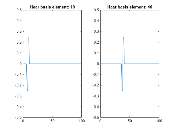
To plot all the wavelet basis elements, set showAll to true.

showAll = false;
if showAll
    figure
    for k=1:100
        plot(xmatHaar(:,k))
        title("Haar basis element: " + num2str(k))
        ylim([-0.5 0.5])
        pause(0.1)
    end
end

Visualize DCT-II

Extract the 100-by-100 submatrix associated with the DCT-II basis.

xmatDCT = subdict(xdict,1:100,101:200);

Display the matrix.

figure
imagesc(xmatDCT)
colormap(gray)
title("DCT-II Basis")

Choose and plot four basis elements.

belement = [10 40 60 90];
for k=1:4
    subplot(2,2,k)
    plot(xmatDCT(:,belement(k)))
    title("DCT-II basis element: " + num2str(belement(k)))
    ylim([-0.5 0.5])
end

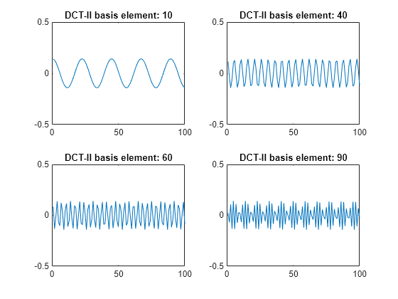
To plot all the DCT-II basis elements, set showAll to true.

showAll = false;
if showAll
    figure
    for k=1:100
        plot(xmatDCT(:,k))
        title("DCT-II basis element: " + num2str(k))
        ylim([-0.5 0.5])
        pause(0.1)
    end
end

Orthogonal Matching Pursuit on 1-D Signal

This example shows how to perform orthogonal matching pursuit on a 1-D input signal that contains a cusp.

Load the cuspamax signal. Construct a dictionary consisting of Daubechies extremal phase wavelets at level 2 and the DCT-II basis.

load cuspamax
lsig = length(cuspamax);
A = sensingDictionary(Size=lsig, ...
    Type={'dwt','dct'}, ...
    Name={'db4'},Level=[2 0]);

Use orthogonal matching pursuit to obtain an approximation of the signal in the sensing dictionary with 100 iterations.

[Xr,YI,I,R] = matchingPursuit(A,cuspamax, ...
    maxIterations=100, ...
    Algorithm="OMP",maxerr={"L2",1});

Extract the vectors from the dictionary that correspond to the approximation. Multiply with the associated coefficients and confirm the result is equal to the approximation.

sMat = subdict(A,1:1024,I);
x = sMat*Xr(I,:);
max(abs(x-YI))

ans = 
0

Plot the signal, approximation, and residual.

subplot(2,1,1)
plot(cuspamax)
hold on
plot(YI)
hold off
legend("Signal","Approx.")
title("Signal and Approximation")
axis tight
subplot(2,1,2)
plot(R)
title("Residual")
axis tight

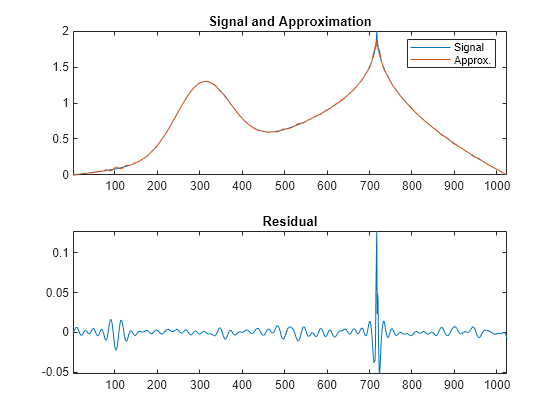
Plot the proportion of retained signal energy for each iteration in the matching pursuit result.

cuspEnergy = cuspamax*cuspamax';
leni = length(I);
recEnergy = zeros(1,leni);
basisElts = subdict(A,1:1024,I);
for k=1:leni
    rec = basisElts(:,1:k)*Xr(I(1:k),:);
    recEnergy(k) = norm(rec)^2/cuspEnergy;
end
figure
plot(recEnergy)
title("Quality / Iteration")
xlabel("Iteration")
ylabel("Quality")

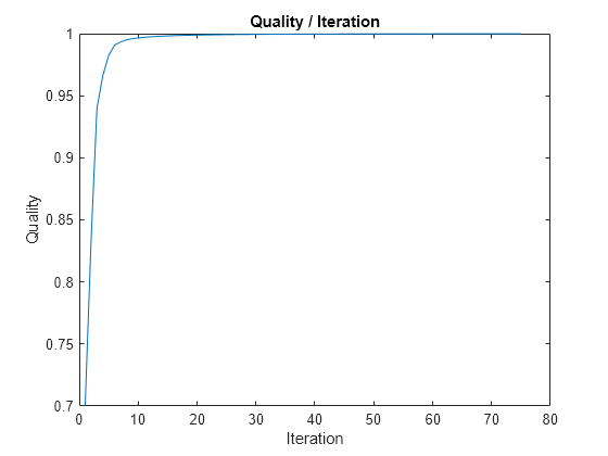
Electricity Consumption Analysis Using Matching Pursuit

This example shows how to compare matching pursuit with a nonlinear approximation in the discrete Fourier transform basis. The data is electricity consumption data collected over a 24-hour period. The example demonstrates that by selecting vectors from a dictionary, matching pursuit is often able to approximate a signal more efficiently with M vectors than any single basis.

Matching Pursuit Using DCT, Fourier, and Wavelet Dictionaries

Load the dataset and plot the data. The dataset contains 35 days of electric consumption. Choose day 32 for further analysis. The data is centered and scaled, so the actual units of usage are not relevant.

load elec35_nor
x = signals(32,:);

plot(x)
xlabel('Minutes')
ylabel('Usage')

The electricity consumption data contains smooth oscillations punctuated by abrupt increases and decreases in usage.

Zoom in on a time interval from 500 minutes to 1200 minutes.

xlim([500 1200])

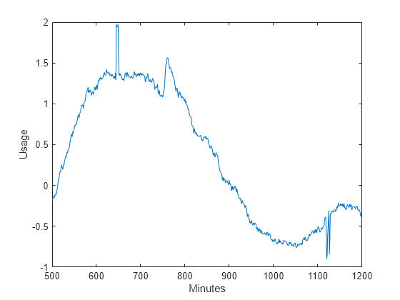
You can see the abrupt changes in the slowly-varying signal at approximately 650, 760, and 1120 minutes. In many real-world signals like these data, the interesting and important information is contained in the transients. It is important to model these transient phenomena.

Construct a signal approximation using 50 vectors chosen from a dictionary with orthogonal matching pursuit (OMP). The dictionary consists of the Haar wavelet at level 2, the discrete cosine transform (DCT) basis, a Fourier basis, and the Kronecker delta basis. Then, use OMP to find the best 50-term greedy approximation of the electric consumption data. Plot the result.

Dict = sensingDictionary('Size',length(x), ...
    'Type',{'dwt','dct','fourier','eye'}, ...
    'Name',{'db1'}, ...
    'Level',[2]);
[Xr,YI,I,R] = matchingPursuit(Dict,x, ...
    maxIterations=50, ...
    Algorithm="OMP",maxerr={"L2",1});

plot(x)
hold on
plot(real(YI))
hold off
xlabel('Minutes')
ylabel('Usage')
legend('Original Signal','OMP')

You can see that with 50 coefficients, orthogonal matching pursuit approximates both the smoothly-oscillating part of the signal and the abrupt changes in electricity usage.

Determine how many vectors the OMP algorithm selected from each of the subdictionaries.

for k=1:4
    basezind{k} = (k-1)*1440+(1:1440);
end
dictvectors = cellfun(@(x)intersect(I,x),basezind,'UniformOutput',false);
for k=1:4
    fprintf("Subdictionary %d: %d vectors\n",k,numel(dictvectors{k}));
end

Subdictionary 1: 0 vectors
Subdictionary 2: 40 vectors
Subdictionary 3: 2 vectors
Subdictionary 4: 8 vectors

The majority of the vectors come from the DCT and Fourier basis. Given the overall slowly-varying nature of the electricity consumption data, this is expected behavior. The additional vectors capture the abrupt signal changes.

Matching Pursuit Using DCT vs. Full Dictionary

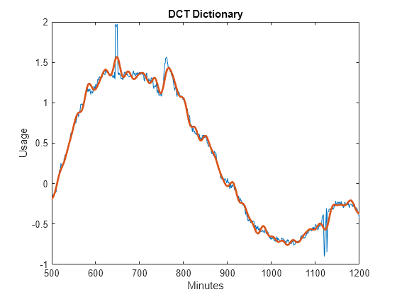
Repeat the OMP with only the DCT subdictionary. Set the OMP to select the 50 best vectors from the DCT dictionary. Construct the dictionary and perform the OMP. Compare the OMP with the DCT dictionary to the OMP with the additional subdictionaries. Notice that adding the Kronecker delta subdictionary shows the abrupt changes in electricity usage more accurately. The advantage of including the Kronecker delta basis is especially clear especially in approximating the upward and downward spikes in usage at approximately 650 and 1120 minutes.

Dict2 = sensingDictionary('Size',length(x),'Type',{'dct'});
[Xr2,YI2,I2,R2] = matchingPursuit(Dict2,x, ...
    maxIterations=50, ...
    Algorithm="OMP",maxerr={"L2",1});

plot(x)
hold on
plot(real(YI2),'linewidth',2)
hold off
title('DCT Dictionary')
xlabel('Minutes')
ylabel('Usage')
xlim([500 1200])

figure
plot(x)
hold on
plot(real(YI),'linewidth',2)
hold off
xlim([500 1200])
title('Full Dictionary')
xlabel('Minutes')
ylabel('Usage')

Obtain the best 50-term nonlinear approximation of the signal in the discrete Fourier basis. Obtain the DFT of the data, sort the DFT coefficients, and select the 50 largest coefficients. The DFT of a real-valued signal is conjugate symmetric, so only consider frequencies from 0 (DC) to the Nyquist (1/2 cycles/minute).

xdft = fft(x);
[~,I] = sort(xdft(1:length(x)/2+1),'descend');
ind = I(1:50);

Examine the vector ind. None of the indices correspond to 0 or the Nyquist. Add the corresponding complex conjugate to obtain the nonlinear approximation in the DFT basis. Plot the approximation and the original signal.

indconj = length(xdft)-ind+2;
ind = [ind indconj];
xdftapp = zeros(size(xdft));
xdftapp(ind) = xdft(ind);
xrec = ifft(xdftapp);

plot(x)
hold on
plot(xrec,'LineWidth',2)
hold off
xlabel('Minutes')
ylabel('Usage')
legend('Original Signal','Nonlinear DFT Approximation')

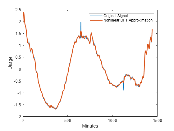
Similar to the DCT dictionary, the nonlinear DFT approximation performs well at matching the smooth oscillations in electricity consumption data. However, the nonlinear DFT approximation does not approximate the abrupt changes accurately. Zoom in on the interval of the data containing the abrupt changes in consumption.

plot(x)
hold on
plot(xrec,'LineWidth',2)
hold off
xlabel('Minutes')
ylabel('Usage')
legend('Original Signal','Nonlinear DFT Approximation')
xlim([500 1200])