Aerodynamic Parameter Estimation Using Flight Log Data
This example shows how to improve the accuracy of a UAV model by using flight log data to estimate its aerodynamic parameters.
Identify Flight Log Time Interval
Open the Flight Log Analyzer app:
flightLogAnalyzer
To visualize the flight log data:
On the app toolstrip, select Import and click From ULOG.
In the Import a ULOG File dialog box, select the
quadrotor_model.ulg fileand click Open.In the Plot section of the app toolstrip, click Add Figure, and select the Height and IMU plots from the gallery.
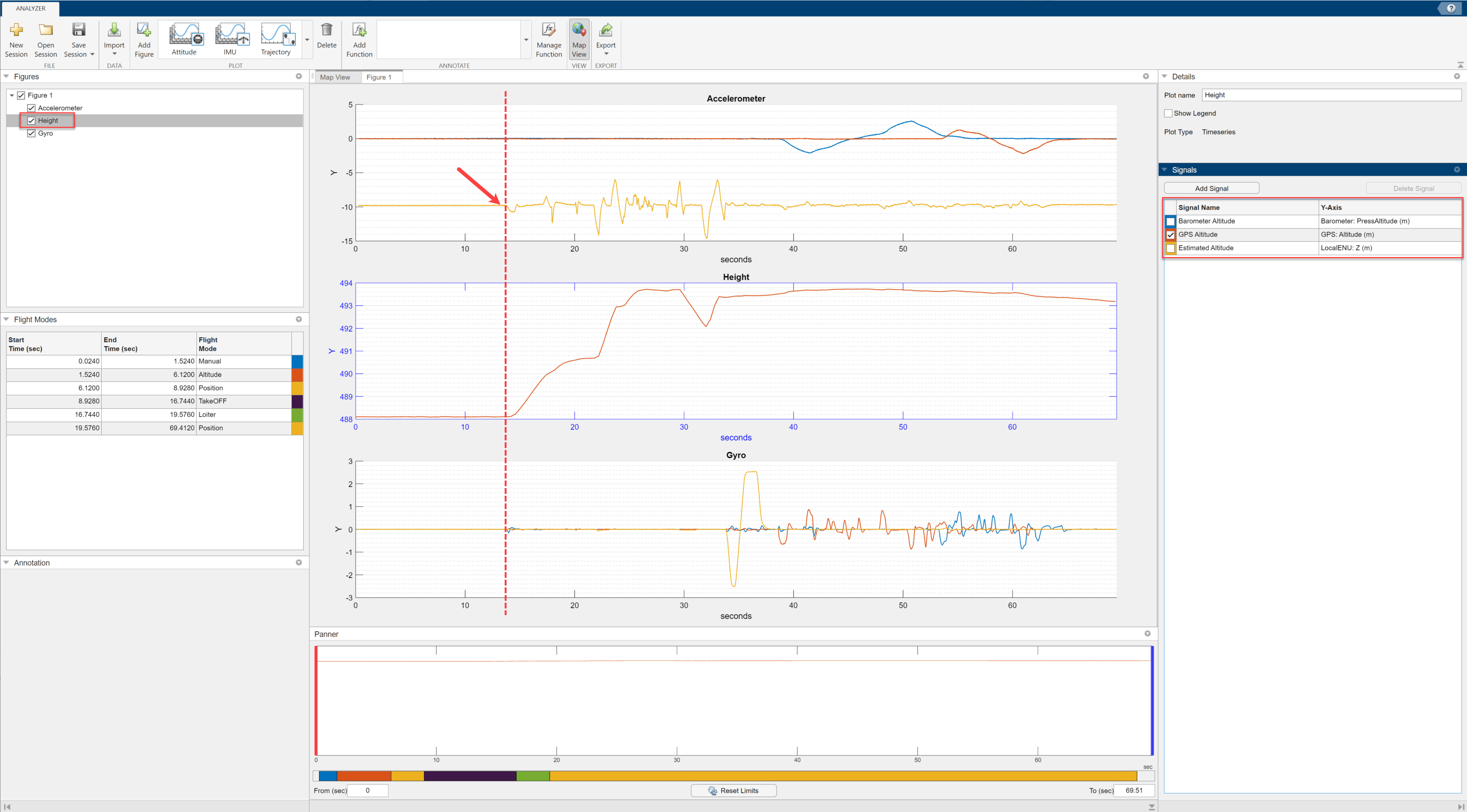
In the Figures pane, select Height.
In the Signals pane, clear the
Barometer AltitudeandEstimated Altitudesignals.
Use the Panner to limit the flight log plot to a time interval of 13.55 to 68 seconds. Observe that, in this interval, the height plot indicates that the UAV takes off, and the accelerometer and gyro plots show significant activity.

Store the time interval.
tStart = 13.55;
tEnd = 68;
Process Flight Log Data
The parameter estimation process uses the flight log data to obtain the inputs to the UAV plant model, and as a ground truth to compare against the output of the plant model. The parameter estimation process requires these types of data from the flight log, formatted as a timetables:
Translational acceleration
Angular acceleration
Translational velocity in the body frame
Angular velocity
Actuator output
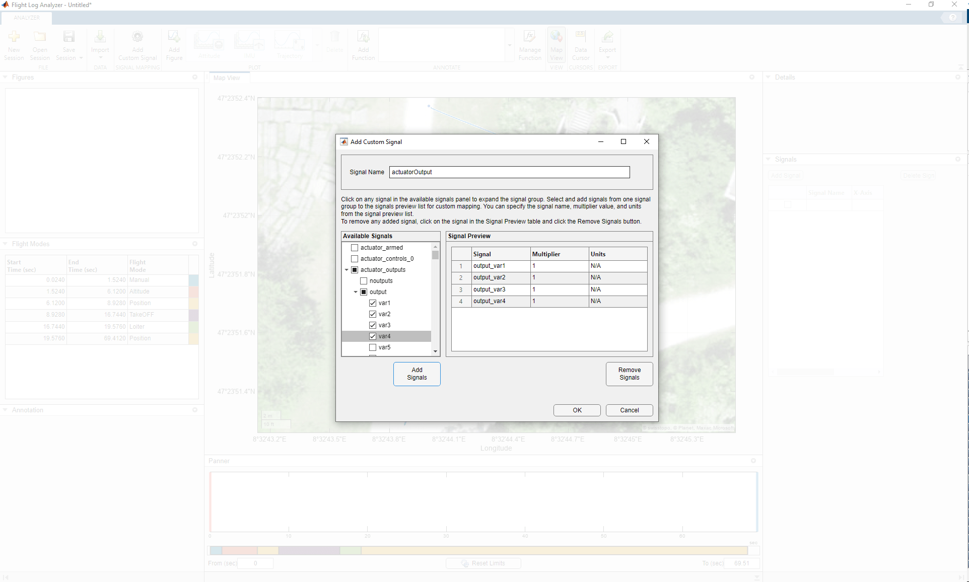
To obtain the signals, from Flight Log Analyzer app toolstrip, select Add Custom Signal. In the Add Custom Signal dialog box:
Specify the signal name as
actuatorOutput.In the Available Signals pane, expand
actuator_outputs, thenoutputs, and select thevar1,var2,var3, andvar4 signalsfromactuator_outputs/output.Click Add Signals.
Click OK.
From the app toolstrip, select Export, then Export Signal. In the dialog box:
In the Select signals to export section, select
actuatorOutput.Select Time Cropping and specify From(sec) as
13.55and To(sec) as 68 seconds.Select Sampling Rate(Hz) and specify the value as
100.Select To MATLAB workspace.
Click Export.
Because the signal export process can take some time, you can instead load a pregenerated exported signal for this example. To get the pregenerated signal, load the exportedSignals.mat file.
load exportedSignals.matSpecify timestamps to use to create timetables.
deltaT = 1/100;
tSample = tStart:deltaT:tEnd;
The exported signal already contains a timetable for translational acceleration. To obtain the timetable for angular acceleration, you must differentiate the angular velocity signal.
ang_acc_x_T = timetable(seconds(tSample'),gradient(vehicle_AngularVelocity_xyz_var1.Var1)./deltaT);
ang_acc_y_T = timetable(seconds(tSample'),gradient(vehicle_AngularVelocity_xyz_var2.Var1)./deltaT);
ang_acc_z_T = timetable(seconds(tSample'),gradient(vehicle_AngularVelocity_xyz_var3.Var1)./deltaT);
Create a timetable for the angular velocity.
ang_vel_T = timetable(seconds(tSample'),[vehicle_AngularVelocity_xyz_var1.Var1 vehicle_AngularVelocity_xyz_var2.Var1 vehicle_AngularVelocity_xyz_var3.Var1]);
Create a timetable of the actuator output.
actuatorOutput = timetable(seconds(tSample'),[actuatorOutput_output_var1.Var1 actuatorOutput_output_var2.Var1 actuatorOutput_output_var3.Var1 actuatorOutput_output_var4.Var1]);

% Set the actuator limits to a minimum value of 1000 and maximum value of 2000, to normalize the actuator inputs between 0 and 1.
n_Actuator_Inputs = normalizeActuators(actuatorOutput.Var1,1000,2000);
n_Actuator_T = timetable(seconds(tSample'),n_Actuator_Inputs);
To get the translational velocity of the UAV in the body frame, first obtain the UAV attitude from the flight log.
ug = ulogreader("quadrotor_model.ulg");
attitudeData = readTopicMsgs(ug,TopicName="vehicle_attitude");
timeAttitude = seconds(attitudeData.TopicMessages{1}.timestamp);
vehicleAttitude = timeseries(attitudeData.TopicMessages{1}.q,timeAttitude);
Use the interp1 function to resample the UAV attitude data at the timetable timestamps.
quatData = interp1(vehicleAttitude.Time,vehicleAttitude.Data,tSample);
Convert the ground speed in the flight log to the body frame by using the orientation data for each time step.
VNED = zeros(length(tSample),3);
Vb = zeros(length(tSample),3);
for ti = 1:1:length(tSample)
    % Get velocity in NED frame at current time step
    VNED(ti,1:3) = [velocityNED_vx.Var1(ti) velocityNED_vy.Var1(ti) velocityNED_vz.Var1(ti)] ;
    % Calculate body velocity using orientation data and velocity in NED
    % frame assuming zero wind
    q = quaternion([quatData(ti,1) quatData(ti,2) quatData(ti,3) quatData(ti,4)]);
    Vb(ti,1:3) = rotateframe(q,VNED(ti,1:3));
end

% Convert the body velocity into the timetable format.
Vb_T = timetable(seconds(tSample'),Vb);
Model Overview
Open the UAVQuadDynamics.slx model.
open_system("UAVQuadDynamics.slx")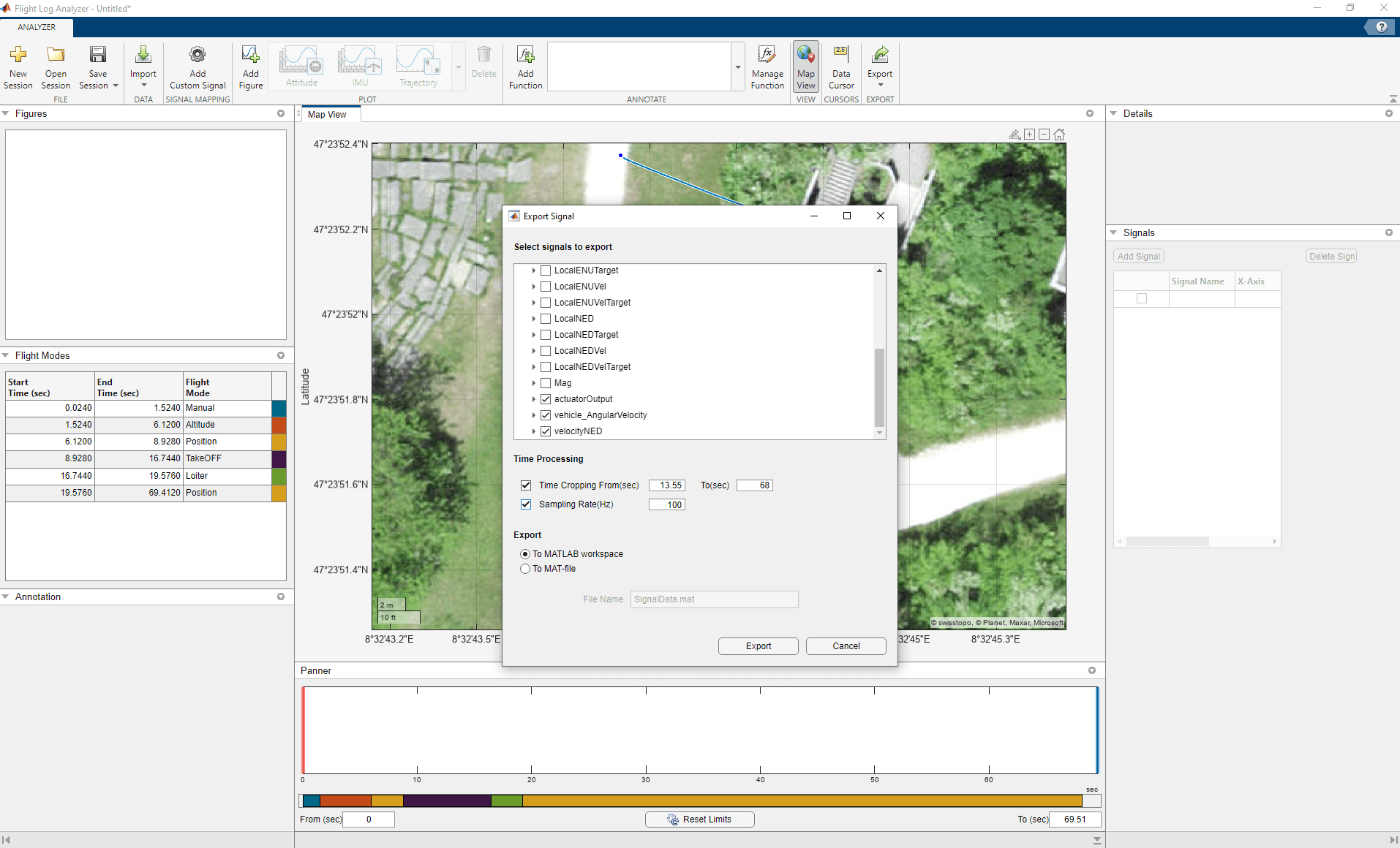
Plant Model
The Plant Model subsystem calculates the translational and angular acceleration response based on a mathematical model of a quadcopter UAV [1]. The Plant Model subsystem receives the system inputs, geometric configuration, and aerodynamic parameters of the UAV.
System Inputs
The System Inputs subsystem outputs these signals for the plant model subsystem:
Vb—UAV Velocity in the body frame, generated using theVb_Ttimetable.Omega—Angular velocity, generated using theang_vel_Ttimetable.actuators—Actuator output, generated using then_Actuator_Ttimetable.
Geometry Configuration
The Geometry Configuration subsystem contains the geometric parameters of the UAV, such as its rotor turn direction, motor positions, and inertia. These parameters remain constant during the parameter estimation process.
Aerodynamic Parameters
The Aerodynamic Parameters subsystem contains the parameters that the plant model subsystem uses to calculate the aerodynamic forces on the UAV. This table summarizes the coefficients:
Coefficient | Description |
|---|---|
| Rotor drag coefficient |
| Rotor thrust coefficient |
| Rotor thrust coefficient at zero advance ratio |
| Fuselage drag coefficient |
| Rotor thrust moment coefficient |
| Rotor thrust moment coefficient at zero advance ratio |
| Rotor drag moment coefficient |
| Rotor drag moment coefficient at zero advance ratio |
| Rotor rolling moment coefficient |
The parameter estimation process estimates these parameters. To start the estimation process, first provide baseline aerodynamic parameters as an initial guess.
CD = 0.06;
CT1 = -0.05;
CT0 = 2;
CDFuselage = [0.025 0.025 0.025];
CM0 = 1.5;
CM1 = -0.01;
CDM0 = 0.15;
CDM1 = -0.04;
CRM = 0.01;
Verify Baseline Aerodynamic Parameters
Simulate the UAVQuadDynamics.slx model using the baseline aerodynamic parameters, and store the output in the MATLAB® workspace as simOutBaseline.
simOutBaseline = sim("UAVQuadDynamics.slx");### Searching for referenced models in model 'UAVQuadDynamics'. ### Total of 2 models to build. ### Starting serial model build. ### Successfully updated the model reference simulation target for: RotorDragMoment ### Successfully updated the model reference simulation target for: ThrustForceModel Build Summary Model reference simulation targets: Model Build Reason Status Build Duration =================================================================================================================== RotorDragMoment Target (RotorDragMoment_msf.mexa64) did not exist. Code generated and compiled. 0h 0m 25.045s ThrustForceModel Target (ThrustForceModel_msf.mexa64) did not exist. Code generated and compiled. 0h 0m 9.7884s 2 of 2 models built (0 models already up to date) Build duration: 0h 0m 41.156s
Plot the X-, Y-, and Z- acceleration responses for both the model and the flight log. The plots show that, when using the baseline aerodynamic parameters, the acceleration responses of the model do not align with the flight log data. This discrepancy indicates that the baseline aerodynamic parameters are not an accurate estimate of the aerodynamic characteristics of the actual UAV.
figure
tiledlayout(3,1)
nexttile
plot(simOutBaseline.tout,simOutBaseline.yout{1}.Values.Data(:),LineWidth=2)
hold on
plot(seconds(Accel_AccelX.Time),Accel_AccelX.Var1)
hold off
xlabel("Time (s)")
ylabel("X (m/s^2)")
legend("Simulated","Flight Log",Location="northwest")
grid on
title("Acceleration Response")

nexttile
plot(simOutBaseline.tout,simOutBaseline.yout{2}.Values.Data(:),LineWidth=2)
hold on
plot(seconds(Accel_AccelY.Time),Accel_AccelY.Var1)
hold off
xlabel("Time (s)")
ylabel("Y (m/s^2)")
legend("Simulated","Flight Log",Location="northwest")
grid on

nexttile
plot(simOutBaseline.tout,simOutBaseline.yout{3}.Values.Data(:),LineWidth=2)
hold on
plot(seconds(Accel_AccelZ.Time),Accel_AccelZ.Var1)
hold off
xlabel("Time (s)")
ylabel("Z (m/s^2)")
legend("Simulated","Flight Log",Location="northeast")
grid on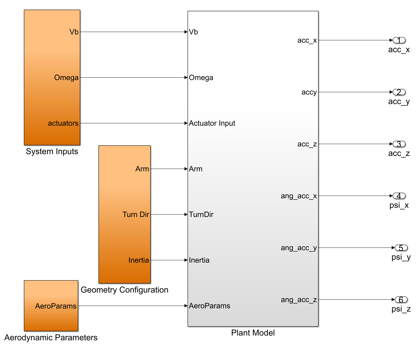
Automatic Tuning of Aerodynamic Parameter
The parameterEstimationUAVQuadDynamics script, attached to this example as a supporting file, enables you to automatically improve the aerodynamic parameter without having to perform multiple simulations to iterate each of the nine parameters.
Run this code in the Command Window to use the parameterEstimationUAVQuadDynamics script and update the parameters in the workspace.
% Tune the parameters
[pOpt,Info] = parameterEstimationQuadrotorDynamics;
% Update the parameters in the workspace using the tuned parameters in pOpt
for i = 1:1:length(pOpt)
    eval(strcat(pOpt(i).Name,"=","[",num2str(pOpt(i).Value),"]"))
end
Because the automatic tuning process can take some time, you can instead load a pre-generated tuning result for this example. To get the pregenerated tuning result, load the tunedParams.mat file.
load tunedParams.matThe tuning process returns these estimated parameters:
Parameter | Value |
|---|---|
|
|
|
|
|
|
|
|
|
|
|
|
|
|
|
|
|
|
The parameterEstimationQuadrotorDynamics script that this example uses has been created using the Parameter Estimator (Simulink Design Optimization) app. For more information on how to load the Parameter Estimator app session used to create the script, see Load Parameter Estimator App Session.
Verify Tuned Aerodynamic Parameters
Simulate the UAVQuadDynamics.slx model using the tuned aerodynamic parameters, and store the output in the MATLAB workspace as simOut.
simOut = sim("UAVQuadDynamics.slx");### Searching for referenced models in model 'UAVQuadDynamics'. ### Total of 2 models to build. ### Model reference simulation target for RotorDragMoment is up to date. ### Model reference simulation target for ThrustForceModel is up to date. Build Summary 0 of 2 models built (2 models already up to date) Build duration: 0h 0m 0.96968s
Plot the X-, Y-, and Z- acceleration responses for both the model and the flight log. The plots show that, when using the tuned aerodynamic parameters, the acceleration responses of the model match those of the flight log data. This alignment indicates that the tuned aerodynamic parameters are an accurate estimate of the aerodynamic characteristics of the actual UAV.
figure
tiledlayout(3,1)
nexttile
plot(simOut.tout,simOut.yout{1}.Values.Data(:),LineWidth=2)
hold on
plot(seconds(Accel_AccelX.Time),Accel_AccelX.Var1)
hold off
xlabel("Time (s)")
ylabel("X (m/s^2)")
legend("Simulated","Flight Log",Location="northwest")
grid on
title("Acceleration Response")

nexttile
plot(simOut.tout,simOut.yout{2}.Values.Data(:),LineWidth=2)
hold on
plot(seconds(Accel_AccelY.Time),Accel_AccelY.Var1)
hold off
xlabel("Time (s)")
ylabel("Y (m/s^2)")
legend("Simulated","Flight Log",Location="northwest")
grid on

nexttile
plot(simOut.tout,simOut.yout{3}.Values.Data(:),LineWidth=2)
hold on
plot(seconds(Accel_AccelZ.Time),Accel_AccelZ.Var1)
hold off
xlabel("Time (s)")
ylabel("Z (m/s^2)")
legend("Simulated","Flight Log",Location="northeast")
grid on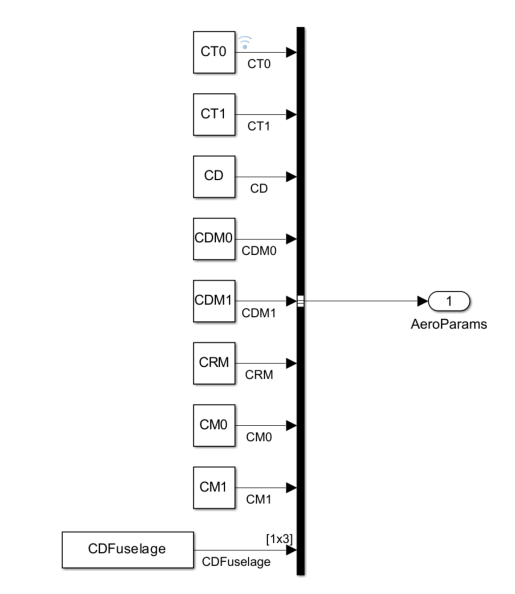
Calculate the root mean squared error of the acceleration data to evaluate the fit of the simulation result to the flight log data.
RMSE_Acc_X = sqrt(mean((Accel_AccelX.Var1 - simOut.yout{1}.Values.Data(:)).^2))RMSE_Acc_X = 0.0314
RMSE_Acc_Y = sqrt(mean((Accel_AccelY.Var1 - simOut.yout{2}.Values.Data(:)).^2))RMSE_Acc_Y = 0.0431
RMSE_Acc_Z = sqrt(mean((Accel_AccelZ.Var1 - simOut.yout{3}.Values.Data(:)).^2))RMSE_Acc_Z = 0.1975
Load Parameter Estimator App Session
To load the Parameter Estimator app session used to create the script, first launch the Parameter Estimator app using this command
spetool("UAVQuadDynamics")
After you open the app:
From the app toolstrip, select Open Session.
Select the
flightdata_spesessionfile.Select Open.
References
[1] Galliker, Manuel Yves. "Data-Driven Dynamics Modelling Using Flight Logs." June 24, 2021. https://doi.org/10.3929/ETHZ-B-000507495.
Copyright 2022 The MathWorks, Inc.
See Also
Flight Log Analyzer | flightLogSignalMapping | ardupilotreader