ラプラス演算子の固有値

この例では、L 型領域でラプラス演算子の固有値問題を解く方法を説明します。

膜の問題

平面内の領域 $Ω$ の境界 $\partial Ω$ に固定されている膜について考えます。その変位 $u (x, y)$ は、固有値問題 $Δ u = λ u$ によって表されます。ここで、 $Δ u = u_{x x} + u_{y y}$ はラプラス演算子、 $λ$ はスカラーパラメーターです。すべての $(x, y) \in \partial Ω$ における境界条件は、 $u (x, y) = 0$ です。

ラプラス演算子は自己共役かつ負定値です。つまり、負の実数固有値 $λ$ のみが存在します。(負の) 最大離散固有値があり、対応する固有関数 $u$ は "基底状態" と呼ばれます。この例では、 $Ω$ は L 型領域であり、この領域に関連付けられた基底状態は L 型膜 (つまり MATLAB® ロゴ) になります。

9 点有限差分法による近似

固有値問題を解く最も簡単な方法は、ラプラシアン $Δ u$ を、 $x$ 方向の距離 hx と $y$ 方向の距離 hy の点から成る正方格子において、有限差分近似 ("ステンシル") により近似することです。この例では、 $Δ u$ を、中点 $(x, y)$ 周辺にある 9 個の一定間隔の格子点の和 S_h を使用して近似します。重み $a_{- 1 - 1}, \dots, a_{11}$ は未知数です。

syms u(x,y) Eps a11 a10 a1_1 a01 a00 a0_1 a_11 a_10 a_1_1
syms hx hy positive
S_h = a_11 * u(x - Eps*hx,y + Eps*hy) +...
      a01  * u(x,y + Eps*hy) +...
      a11  * u(x + Eps*hx,y + Eps*hy) +... 
      a_10 * u(x - Eps*hx,y) +... 
      a00  * u(x,y) +... 
      a10  * u(x + Eps*hx,y) +...
      a_1_1* u(x - Eps*hx,y - Eps*hy) +...
      a0_1 * u(x,y - Eps*hy) +...
      a1_1 * u(x + Eps*hx,y - Eps*hy);

シンボリックパラメーター Eps を使用して、この式の展開を hx と hy のべき乗で並べ替えます。重みがわかると、Eps = 1 を設定してラプラシアンを近似できます。

t = taylor(S_h, Eps, 'Order', 7);

関数 coeffs を使用して、Eps のべき乗が同じ項の係数を抽出します。各係数は、hx、hy のべき乗および $x$ と $y$ に対する u の導関数を含む式です。S_h は、 $u_{x x} + u_{y y}$ であるため、その他すべての u の導関数の係数は 0 でなければなりません。 $u_{x x}$ と $u_{y y}$ を除く u のすべての導関数を 0 に置き換えて係数を抽出します。 $u_{x x}$ と $u_{y y}$ を 1 に置き換えます。これにより、テイラー展開が計算する係数に簡約され、以下の 6 つの線形方程式が導かれます。

C = formula(coeffs(t, Eps, 'All'));
eq0  = subs(C(7),u(x,y),1) == 0;
eq11 = subs(C(6),[diff(u,x),diff(u,y)],[1,0]) == 0;
eq12 = subs(C(6),[diff(u,x),diff(u,y)],[0,1]) == 0;
eq21 = subs(C(5),[diff(u,x,x),diff(u,x,y),diff(u,y,y)],[1,0,0]) == 1;
eq22 = subs(C(5),[diff(u,x,x),diff(u,x,y),diff(u,y,y)],[0,1,0]) == 0;
eq23 = subs(C(5),[diff(u,x,x),diff(u,x,y),diff(u,y,y)],[0,0,1]) == 1;

S_h には 9 つの未知の重みがあるため、u のすべての 3 次導関数を 0 とする要件によってさらに方程式を追加します。

eq31 = subs(C(4),[diff(u,x,x,x),diff(u,x,x,y),diff(u,x,y,y),diff(u,y,y,y)], [1,0,0,0]) == 0;
eq32 = subs(C(4),[diff(u,x,x,x),diff(u,x,x,y),diff(u,x,y,y),diff(u,y,y,y)], [0,1,0,0]) == 0;
eq33 = subs(C(4),[diff(u,x,x,x),diff(u,x,x,y),diff(u,x,y,y),diff(u,y,y,y)], [0,0,1,0]) == 0;
eq34 = subs(C(4),[diff(u,x,x,x),diff(u,x,x,y),diff(u,x,y,y),diff(u,y,y,y)], [0,0,0,1]) == 0;

9 つの未知の重みに対して、得られた 10 個の方程式を解きます。ReturnConditions を使用して、任意のパラメーターを含むすべての解を求めます。

[a11,a10,a1_1,a01,a00,a0_1,a_11,a_10,a_1_1,parameters,conditions] = ...
    solve([eq0,eq11,eq12,eq21,eq22,eq23,eq31,eq32,eq33,eq34], ...
          [a11,a10,a1_1,a01,a00,a0_1,a_11,a_10,a_1_1], ...
          'ReturnConditions',true);

expand([a_11,a01,a11;...
        a_10,a00,a01;...
        a1_1,a0_1,a_1_1])

ans = 
 $(\begin{array}{c} z & \frac{1}{{hy}^{2}} - 2 z & z \\ \frac{1}{{hx}^{2}} - 2 z & 4 z - \frac{2}{{hx}^{2}} - \frac{2}{{hy}^{2}} & \frac{1}{{hy}^{2}} - 2 z \\ z & \frac{1}{{hy}^{2}} - 2 z & z \end{array})$

parameters

parameters =  $z$

関数 subs を使用して、重みをそれぞれの計算値に置き換えます。

C = simplify(subs(C));

u の 0 次、1 次および 3 次の導関数を含む式 C(7)、C(6) および C(4) は消えます。

[C(7), C(6), C(4)]

ans =  $(\begin{array}{c} 0 & 0 & 0 \end{array})$

式 C(5) は u のラプラシアンになります。

C(5)

ans = 
 $\frac{\partial^{2}}{\partial x^{2}} u (x, y) + \frac{\partial^{2}}{\partial y^{2}} u (x, y)$

したがって、上で計算された重みの値を使用すると、ステンシル S_h は、任意のパラメーター z のどの値についても最大次数 hx^2、hy^2 のラプラシアンを近似します。ただし、z には次数 O(1/hx^2,1/hy^2) が選ばれている場合に限ります。

4 次以上の導関数を含む項

解に自由パラメーター z が含まれていますが、u の 4 次導関数を含む式 C(3) は、z の適切な選択によって 0 にすることができません。別の選択肢として、ラプラス演算子の 2 乗の倍数にする方法があります。

syms d
Laplace = @(u) laplacian(u,[x,y]);
expand(d*Laplace(Laplace(u)))

ans(x, y) = 
 $d \frac{\partial^{4}}{\partial x^{4}} u (x, y) + 2 d \frac{\partial^{2}}{\partial y^{2}} \frac{\partial^{2}}{\partial x^{2}} u (x, y) + d \frac{\partial^{4}}{\partial y^{4}} u (x, y)$

C(3) の u の各導関数を選択して、それらの係数を対応する項と等式化します。

subs(C(3),[diff(u,x,x,x,x),diff(u,x,x,y,y),diff(u,y,y,y,y)],[1,0,0]) == d

ans = 
 $\frac{{hx}^{2}}{12} = d$

subs(C(3),[diff(u,x,x,x,x),diff(u,x,x,y,y),diff(u,y,y,y,y)],[0,1,0]) == 2*d

ans =  ${hx}^{2} {hy}^{2} z = 2 d$

subs(C(3),[diff(u,x,x,x,x),diff(u,x,x,y,y),diff(u,y,y,y,y)],[0,0,1]) == d

ans = 
 $\frac{{hy}^{2}}{12} = d$

したがって、d = hx^2/12 = hy^2/12 と z = 2*d/(hx^2*hy^2) を選択できます。これは、hx = hy および z = 1/(6*hx*hy) を意味します。そのため、ステンシル S_h は修正したラプラシアンを hx = hy = h の正方格子上で近似します。

$S_{h} = Δ u + \frac{h^{2}}{12} Δ^{2} u + O (h^{3}) . (1)$

syms h
hx = h;
hy = h;
d = h^2/12;

hx と hy を h に置き換えます。

C = subs(C);

z を、その値である 1/(6*h^2) に置き換えます。z は MATLAB ワークスペースに存在しないため、parameters 配列に保存された値でのみ利用できます。

C = subs(C,parameters,1/(6*h^2));

式 (1) を検証します。

simplify(C(3) - d*Laplace(Laplace(u)))

ans(x, y) =  $0$

次に、hx、hy の 3 次の項について考えます。

simplify(C(2))

ans =  $0$

ステンシルの展開にはこの項が存在しないため、(1) の項 $O (h^{3})$ は事実上、次数 $O (h^{4})$ になります。ステンシルの 4 次の項について考えます。

factor(simplify(C(1)))

ans = 
 $(\begin{array}{c} \frac{1}{360} & h & h & h & h & \frac{\partial^{6}}{\partial x^{6}} u (x, y) + 5 \frac{\partial^{2}}{\partial y^{2}} \frac{\partial^{4}}{\partial x^{4}} u (x, y) + 5 \frac{\partial^{4}}{\partial y^{4}} \frac{\partial^{2}}{\partial x^{2}} u (x, y) + \frac{\partial^{6}}{\partial y^{6}} u (x, y) \end{array})$

これらの項がラプラス演算子のさらに別のべき乗でも特定できるかを確認します。しかし、以下との比較では

Laplace(Laplace(Laplace(u)))

ans(x, y) = 
 $\frac{\partial^{6}}{\partial x^{6}} u (x, y) + 3 \frac{\partial^{2}}{\partial y^{2}} \frac{\partial^{4}}{\partial x^{4}} u (x, y) + 3 \frac{\partial^{4}}{\partial y^{4}} \frac{\partial^{2}}{\partial x^{2}} u (x, y) + \frac{\partial^{6}}{\partial y^{6}} u (x, y)$

次数 $O (h^{4})$ の式は、係数が一致しないため、ラプラス演算子の 3 乗の倍数として特定できないことが示されています。

まとめ

隣接する格子点間の距離が h の正方格子で、上記のように重みを選択した場合、以下が得られます。

$S_{h} = Δ u + \frac{h^{2}}{12} Δ^{2} u + O (h^{4}) . (2)$

この展開を、固有値問題 $Δ u = λ u$ に対する数値的なアプローチとして利用します。 $Δ^{2} u = λ^{2} u$ の倍数を固有値方程式に加算します。

$Δ u + \frac{h^{2}}{12} Δ^{2} u = (λ + \frac{h^{2}}{12} λ^{2}) u .$

この方程式の左辺は、ステンシル $S_{h}$ で十分に近似されています。したがって、(2) を使用すると、 $S_{h} u = μ u$ を満たすステンシルの数値的固有値 $μ$ は、以下により、ラプラス演算子の固有値 $λ$ の近似でなければなりません。

$μ = λ + \frac{h^{2}}{12} λ^{2} + O (h^{4}) .$

特定の $μ$ に対して、 $λ$ を解き、より適切なラプラス固有値の近似を得ます。 $λ$ の 2 次方程式の解には、 $h \to 0$ の場合に $λ \to μ$ になるという要件によって正しい符号の平方根が定められます。

$λ = \frac{6}{h^{2}} (\sqrt{1 + \frac{μ h^{2}}{3}} - 1) = \frac{2 μ}{\sqrt{1 + \frac{μ h^{2}}{3}} + 1} . (3)$

シンボリック行列を使用した固有値問題の求解

3 つの単位正方形で構成される L 型領域 $Ω$ を考えます。

$Ω = {(x, y); - 1 \leq x \leq 0, - 1 \leq y \leq 0} \cup {(x, y); 0 \leq x \leq 1, - 1 \leq y \leq 0} \cup {(x, y); - 1 \leq x \leq 0, 0 \leq y \leq 1} .$

領域の角の座標値を定義します。

xmin =-1;
xmax = 1; 
ymin =-1; 
ymax = 1;

x 方向の奇数 (Nx=2*nx-1) の格子点と y 方向の奇数 (Ny=2*ny-1) の格子点で構成される正方グリッドを考えます。

nx = 6; 
Nx = 2*nx-1; 
hx = (xmax-xmin)/(Nx-1);

ny = 6; 
Ny = 2*ny-1; 
hy = (ymax-ymin)/(Ny-1);

Ny 行 Nx 列のシンボリック行列 $u$ を作成します。その要素 u(i,j) は、固有値問題 $Δ u = λ u$ の解 u(x,y) の値 u(xmin + (j - 1)*hx,ymin + (i - 1)*hy) を表します。

u = sym('u',[Ny,Nx]);

$Ω$ の境界は以下のインデックスに対応します。

左境界は (i = 1:Ny, j = 1) に対応します。
下限は (i = 1, j = 1:Nx) に対応します。
右境界は (i = 1:ny, j = Nx) と (i = ny:Ny, j = nx) に対応します。
上限は (i = Ny, j =1:nx) と (i = ny, j = nx:Nx) に対応します。

u(:,1) = 0;      % left boundary
u(1,:) = 0;      % lower boundary
u(1:ny,Nx) = 0;  % right boundary, upper part
u(ny:Ny,nx) = 0; % right boundary, lower part
u(Ny,1:nx) = 0;  % upper boundary, left part
u(ny,nx:Nx) = 0; % upper boundary, right part

$0 < x \leq 1$ および $0 < y \leq 1$ の領域は $Ω$ に属しません。対応する行列要素 (i = ny + 1:Ny, j = nx + 1:Nx) を 0 に設定します。これらの影響はないため、無視します。

u(ny + 1:Ny,nx + 1:Nx) = 0;

以下の行列要素が問題の未知数です。

u = 
 $(\begin{array}{c} 0 & 0 & 0 & 0 & 0 & 0 & 0 & 0 & 0 & 0 & 0 \\ 0 & u_{2, 2} & u_{2, 3} & u_{2, 4} & u_{2, 5} & u_{2, 6} & u_{2, 7} & u_{2, 8} & u_{2, 9} & u_{2, 10} & 0 \\ 0 & u_{3, 2} & u_{3, 3} & u_{3, 4} & u_{3, 5} & u_{3, 6} & u_{3, 7} & u_{3, 8} & u_{3, 9} & u_{3, 10} & 0 \\ 0 & u_{4, 2} & u_{4, 3} & u_{4, 4} & u_{4, 5} & u_{4, 6} & u_{4, 7} & u_{4, 8} & u_{4, 9} & u_{4, 10} & 0 \\ 0 & u_{5, 2} & u_{5, 3} & u_{5, 4} & u_{5, 5} & u_{5, 6} & u_{5, 7} & u_{5, 8} & u_{5, 9} & u_{5, 10} & 0 \\ 0 & u_{6, 2} & u_{6, 3} & u_{6, 4} & u_{6, 5} & 0 & 0 & 0 & 0 & 0 & 0 \\ 0 & u_{7, 2} & u_{7, 3} & u_{7, 4} & u_{7, 5} & 0 & 0 & 0 & 0 & 0 & 0 \\ 0 & u_{8, 2} & u_{8, 3} & u_{8, 4} & u_{8, 5} & 0 & 0 & 0 & 0 & 0 & 0 \\ 0 & u_{9, 2} & u_{9, 3} & u_{9, 4} & u_{9, 5} & 0 & 0 & 0 & 0 & 0 & 0 \\ 0 & u_{10, 2} & u_{10, 3} & u_{10, 4} & u_{10, 5} & 0 & 0 & 0 & 0 & 0 & 0 \\ 0 & 0 & 0 & 0 & 0 & 0 & 0 & 0 & 0 & 0 & 0 \end{array})$

領域 $Ω ∖ \partial Ω$ の内側の点は、問題の未知の値 $u (i, j)$ を含むインデックス $(i, j)$ に対応します。これらの未知数をベクトル vars に集めます。

[I,J] = find(u~=0);
vars = u(u~=0);

シンボリック式 (この例の最初の部分で導出したステンシルによって与えられる) と各インデックス (つまり、個々の未知数) を関連付けます。

n = length(vars);
Lu = sym(zeros(n,1));
for k=1:n
   i = I(k);
   j = J(k);
   Lu(k) =   1/6*u(i+1,j-1) +  2/3*u(i+1,j) + 1/6*u(i+1,j+1) ...
           + 2/3*u( i ,j-1) - 10/3*u( i ,j) + 2/3*u( i ,j+1) ...
           + 1/6*u(i-1,j-1) +  2/3*u(i-1,j) + 1/6*u(i-1,j+1); 
end
Lu = Lu/hx^2;

この式は u の未知の要素 (vars に保存) において線形であるため、ベクトル vars に基づく行列として処理できます。

S_h = jacobian(Lu, vars);

S_h はラプラス演算子の行列近似として処理できます。その固有ベクトルと固有値を計算します。

[V,D] = eig(vpa(S_h));

3 つの最大固有値は D の最初の対角要素によって与えられます。

[D(1,1), D(2,2), D(3,3)]

ans =  $(\begin{array}{c} - 9.5214641572625960021345709535953 & - 14.431096242107969492574666743957 & - 18.490392088545609858994660377955 \end{array})$

この近似では、点数が少ない格子を使用したため、固有値の先頭の数字のみが正確です。

L 型領域 $Ω$ で 3 番目に高いラプラス演算子の固有値は、厳密にわかっています。ラプラス演算子の厳密な固有関数は、(厳密な) 固有値 $- 2 π^{2} = - 19.7392 . . .$ に関連付けられた関数 $u (x, y) = \sin (π x) \sin (π y)$ です。実際に、上の方程式 (3) を使用すると、ステンシルの固有値 $μ$ からより適切なラプラスの固有値 $λ$ の近似を導出できます。

mu = D(3,3)

mu =  $- 18.490392088545609858994660377955$

lambda = 2*mu / (sqrt(1 + mu*hx^2/3) + 1)

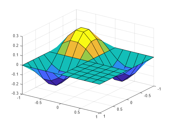
lambda =  $- 19.796765119155672176257649532142$

3 番目に高い固有値に関連付けられた固有関数をプロットします。

v = V(:,3);
for k=1:n
  u(I(k),J(k)) = v(k);
end
u = double(u);
surf(xmin:hx:xmax,ymin:hy:ymax,u');
view(125, 30);

Figure contains an axes object. The axes object contains an object of type surface.

倍精度行列を使用した固有値問題の求解

シンボリック行列を使用する場合、シンボリック計算は MATLAB 倍精度行列による数値計算よりも著しく時間がかかるため、格子点数を大幅に増やすことは推奨されません。この例の部分では、数値上の格子を調整できる倍精度スーパース演算の使用方法を説明します。前述と同様の方法で、L 型領域 $Ω$ を設定します。シンボリックな未知数で内側の点を表すのではなく、格子の値 u を 1 で初期化し、境界点と外側の点を 0 に設定して $Ω$ を定義します。内側の各点のシンボリック式を定義してステンシルをヤコビアンとして計算するのではなく、ステンシル行列を直接、スパース行列として設定します。

xmin =-1; 
xmax = 1; 
ymin =-1; 
ymax = 1;

nx = 30; 
Nx = 2*nx-1; 
hx = (xmax-xmin)/(Nx-1);

ny = 30; 
Ny = 2*ny-1; 
hy = (ymax-ymin)/(Ny-1);

u = ones(Ny,Nx); 
u(:,1) = 0;      % left boundary
u(1:ny,Nx) = 0;  % right boundary, upper part
u(ny:Ny,nx) = 0; % right boundary, lower part
u(1,:) = 0;      % lower boundary
u(Ny,1:nx) = 0;  % upper boundary, left part
u(ny,nx:Nx) = 0; % upper boundary, right part
u(ny + 1:Ny,nx + 1:Nx) = 0;

[I,J] = find(u ~= 0);
n = length(I);
S_h = sparse(n,n);
for k=1:n 
  i = I(k);
  j = J(k);
  S_h(k,I==i+1 & J==j+1)=  1/6;
  S_h(k,I==i+1 & J== j )=  2/3;
  S_h(k,I==i+1 & J==j-1)=  1/6;
  S_h(k,I== i  & J==j+1)=  2/3;
  S_h(k,I== i  & J== j )=-10/3;
  S_h(k,I== i  & J==j-1)=  2/3;
  S_h(k,I==i-1 & J==j+1)=  1/6;
  S_h(k,I==i-1 & J== j )=  2/3;
  S_h(k,I==i-1 & J==j-1)=  1/6;
end
S_h = S_h./hx^2;

ここで、S_h は (スパース) ステンシル行列です。スパース行列を処理する eigs を使用して 3 つの最大固有値を計算します。

[V,D] = eigs(S_h,3,'la');

3 つの最大固有値は D の最初の対角要素です。

[D(1,1), D(2,2), D(3,3)]

ans = 1×3

   -9.6493  -15.1742  -19.7006

D(3,3) は厳密な固有値 $- 2 π^{2} = - 19.7392088 . . .$ に近い値です。上の方程式 (3) を使用すると、ステンシルの固有値 $μ$ からより正確なラプラスの固有値 $λ$ の近似を導出できます。

mu = D(3,3)

mu = -19.7006

lambda = 2*mu / (sqrt(1 + mu*hx^2/3) + 1)

lambda = -19.7393

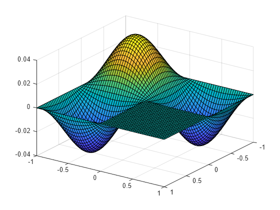
3 番目に高い固有値に関連付けられた固有関数をプロットします。

v = V(:,3);
for k=1:n
  u(I(k),J(k)) = v(k);
end
surf(xmin:hx:xmax, ymin:hy:ymax,u');
view(125, 30);

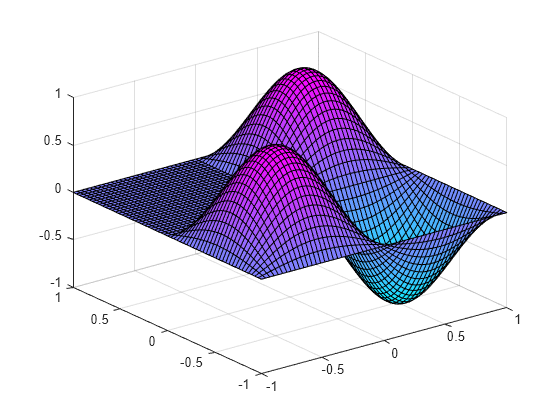
Figure contains an axes object. The axes object contains an object of type surface.

MATLAB 関数 membrane は、ラプラス演算子の固有関数の計算を別の方法で行うことに注意してください。

membrane(3, nx - 1, 8, 8);

Figure contains an axes object. The axes object contains an object of type surface.