アンサンブルの正則化

正則化とは、予測性能を低下させずに、アンサンブルのために選択する弱学習器の数を少なくするプロセスです。現在のところ、正則化できるのはアンサンブル回帰です。(非アンサンブルのコンテキストで判別分析分類器を正則化することもできます。判別分析分類器の正則化を参照してください)。

regularize メソッドは、最小化が可能な学習器の最適な重みのセット α_t を求めます。

$\sum_{n = 1}^{N} w_{n} g ((\sum_{t = 1}^{T} α_{t} h_{t} (x_{n})), y_{n}) + λ \sum_{t = 1}^{T} | α_{t} | .$

ここで、

λ ≥ 0 は、メソッドに渡すパラメーターです。LASSO パラメーターと呼ばれます。
h_t は、予測子 x_n、応答 y_n、および重み w_n をもつ N の観測で学習されたアンサンブルの弱学習器です。
g(f,y) = (f – y)² は二乗誤差です。

アンサンブルは、学習に使用されたのと同じ (x_n,y_n,w_n) データについて正則化されます。そのため、

$\sum_{n = 1}^{N} w_{n} g ((\sum_{t = 1}^{T} α_{t} h_{t} (x_{n})), y_{n})$

は、アンサンブル再代入誤差です。この誤差は平均二乗誤差 (MSE) によって測定されます。

λ = 0 を使用した場合、regularize は再代入 MSE を最小化することにより弱学習器の重みを求めます。アンサンブルには過学習の傾向があります。つまり、再代入誤差は真の汎化誤差より通常は少なくなります。再代入誤差をさらに少なくすることによって、アンサンブルの精度が向上するどころか、逆に低下する結果になりやすいといえます。一方、λ を正の値にすると、α_t 係数の大きさが 0 に近付きます。多くの場合、このようにすると汎化誤差が改善されます。もちろん、大きすぎる λ を選択した場合には、すべての最適係数が 0 になり、アンサンブルの精度は失われます。通常は、正則化されたアンサンブルが正則化されないフルセットのアンサンブルと同等かそれ以上の精度になるような、λ の最適な範囲を求めることができます。

LASSO 正則化には、最適化された係数を正確に 0 にするという便利な特徴があります。学習器の重み α_t が 0 の場合、この学習器を正則化アンサンブルから除外できます。結果的に、精度が高く、学習器の数が少ないアンサンブルが得られることになります。

アンサンブル回帰の正則化

ライブスクリプトを開く

この例では、多くの属性に基づいて、自動車の保険リスクを予測するためのデータを使用します。

imports-85 データを MATLAB® ワークスペースに読み込みます。

load imports-85;

データの説明を参照して、カテゴリカル変数と予測子名を探します。

Description

Description = 9×79 char array
    '1985 Auto Imports Database from the UCI repository                             '
    'http://archive.ics.uci.edu/ml/machine-learning-databases/autos/imports-85.names'
    'Variables have been reordered to place variables with numeric values (referred '
    'to as "continuous" on the UCI site) to the left and categorical values to the  '
    'right. Specifically, variables 1:16 are: symboling, normalized-losses,         '
    'wheel-base, length, width, height, curb-weight, engine-size, bore, stroke,     '
    'compression-ratio, horsepower, peak-rpm, city-mpg, highway-mpg, and price.     '
    'Variables 17:26 are: make, fuel-type, aspiration, num-of-doors, body-style,    '
    'drive-wheels, engine-location, engine-type, num-of-cylinders, and fuel-system. '

このプロセスの目的は、データの最初の変数である "symboling" を他の予測子から予測することです。"symboling" は、-3 (保険リスクが低い) から 3 (保険リスクが高い) までの整数です。ここで、アンサンブル回帰の代わりにアンサンブル分類を使用して、このリスクを予測できる場合もあります。回帰と分類を選択できるケースでは、最初に回帰の使用を試みます。

アンサンブル近似に使用するデータを準備します。

Y = X(:,1);
X(:,1) = [];
VarNames = {'normalized-losses' 'wheel-base' 'length' 'width' 'height' ...
  'curb-weight' 'engine-size' 'bore' 'stroke' 'compression-ratio' ...
  'horsepower' 'peak-rpm' 'city-mpg' 'highway-mpg' 'price' 'make' ...
  'fuel-type' 'aspiration' 'num-of-doors' 'body-style' 'drive-wheels' ...
  'engine-location' 'engine-type' 'num-of-cylinders' 'fuel-system'};
catidx = 16:25; % indices of categorical predictors

300 本の木を使用してデータからアンサンブル回帰を作成します。

ls = fitrensemble(X,Y,'Method','LSBoost','NumLearningCycles',300, ...
    'LearnRate',0.1,'PredictorNames',VarNames, ...
    'ResponseName','Symboling','CategoricalPredictors',catidx)

ls = 
  RegressionEnsemble
           PredictorNames: {1×25 cell}
             ResponseName: 'Symboling'
    CategoricalPredictors: [16 17 18 19 20 21 22 23 24 25]
        ResponseTransform: 'none'
          NumObservations: 205
               NumTrained: 300
                   Method: 'LSBoost'
             LearnerNames: {'Tree'}
     ReasonForTermination: 'Terminated normally after completing the requested number of training cycles.'
                  FitInfo: [300×1 double]
       FitInfoDescription: {2×1 cell}
           Regularization: []


  Properties, Methods

最後の行、Regularization は空 ([]) です。アンサンブルを正則化するには、regularize メソッドを使用しなければなりません。

cv = crossval(ls,'KFold',5);
figure;
plot(kfoldLoss(cv,'Mode','Cumulative'));
xlabel('Number of trees');
ylabel('Cross-validated MSE');
ylim([0.2,2])

Figure contains an axes object. The axes object with xlabel Number of trees, ylabel Cross-validated MSE contains an object of type line.

結果によれば、50 ～ 100 本のツリーで構成されるように、アンサンブルのサイズを小さくすることによって、満足な性能が得られると判断できます。

regularize メソッドを呼び出し、アンサンブルから削除できる木を求めます。既定の設定では、regularize は指数関数的な間隔の LASSO (Lambda) パラメーターの 10 個の値を検査します。

ls = regularize(ls)

ls = 
  RegressionEnsemble
           PredictorNames: {1×25 cell}
             ResponseName: 'Symboling'
    CategoricalPredictors: [16 17 18 19 20 21 22 23 24 25]
        ResponseTransform: 'none'
          NumObservations: 205
               NumTrained: 300
                   Method: 'LSBoost'
             LearnerNames: {'Tree'}
     ReasonForTermination: 'Terminated normally after completing the requested number of training cycles.'
                  FitInfo: [300×1 double]
       FitInfoDescription: {2×1 cell}
           Regularization: [1×1 struct]


  Properties, Methods

ここでは、Regularization プロパティは空ではありません。

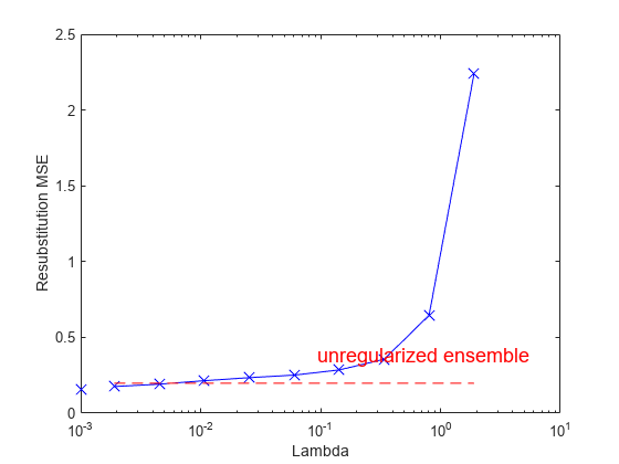
LASSO パラメーターに対して、再代入二乗平均誤差 (MSE) と重みがゼロでない学習器の数をプロットします。Lambda = 0 での値は別にプロットします。Lambda の値は指数関数的な間隔であるため、対数スケールを使用します。

figure;
semilogx(ls.Regularization.Lambda,ls.Regularization.ResubstitutionMSE, ...
    'bx-','Markersize',10);
line([1e-3 1e-3],[ls.Regularization.ResubstitutionMSE(1) ...
     ls.Regularization.ResubstitutionMSE(1)],...
    'Marker','x','Markersize',10,'Color','b');
r0 = resubLoss(ls);
line([ls.Regularization.Lambda(2) ls.Regularization.Lambda(end)],...
     [r0 r0],'Color','r','LineStyle','--');
xlabel('Lambda');
ylabel('Resubstitution MSE');
annotation('textbox',[0.5 0.22 0.5 0.05],'String','unregularized ensemble', ...
    'Color','r','FontSize',14,'LineStyle','none');

Figure contains an axes object. The axes object with xlabel Lambda, ylabel Resubstitution MSE contains 3 objects of type line.

figure;
loglog(ls.Regularization.Lambda,sum(ls.Regularization.TrainedWeights>0,1));
line([1e-3 1e-3],...
    [sum(ls.Regularization.TrainedWeights(:,1)>0) ...
    sum(ls.Regularization.TrainedWeights(:,1)>0)],...
    'marker','x','markersize',10,'color','b');
line([ls.Regularization.Lambda(2) ls.Regularization.Lambda(end)],...
    [ls.NTrained ls.NTrained],...
    'color','r','LineStyle','--');
xlabel('Lambda');
ylabel('Number of learners');
annotation('textbox',[0.3 0.8 0.5 0.05],'String','unregularized ensemble',...
    'color','r','FontSize',14,'LineStyle','none');

Figure contains an axes object. The axes object with xlabel Lambda, ylabel Number of learners contains 3 objects of type line.

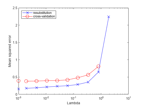
再代入 MSE の値は過度に楽観的になる傾向があります。Lambda のさまざまな値に関連する誤差について信頼性の高い推定を得るには、cvshrink を使用して交差検証を実施します。Lambda に対して、交差検証損失 (MSE) の結果と学習器の数をプロットします。

rng(0,'Twister') % for reproducibility
[mse,nlearn] = cvshrink(ls,'Lambda',ls.Regularization.Lambda,'KFold',5);

Warning: Some folds do not have any trained weak learners.

figure;
semilogx(ls.Regularization.Lambda,ls.Regularization.ResubstitutionMSE, ...
    'bx-','Markersize',10);
hold on;
semilogx(ls.Regularization.Lambda,mse,'ro-','Markersize',10);
hold off;
xlabel('Lambda');
ylabel('Mean squared error');
legend('resubstitution','cross-validation','Location','NW');
line([1e-3 1e-3],[ls.Regularization.ResubstitutionMSE(1) ...
     ls.Regularization.ResubstitutionMSE(1)],...
    'Marker','x','Markersize',10,'Color','b','HandleVisibility','off');
line([1e-3 1e-3],[mse(1) mse(1)],'Marker','o',...
    'Markersize',10,'Color','r','LineStyle','--','HandleVisibility','off');

Figure contains an axes object. The axes object with xlabel Lambda, ylabel Mean squared error contains 2 objects of type line. These objects represent resubstitution, cross-validation.

figure;
loglog(ls.Regularization.Lambda,sum(ls.Regularization.TrainedWeights>0,1));
hold;

Current plot held

loglog(ls.Regularization.Lambda,nlearn,'r--');
hold off;
xlabel('Lambda');
ylabel('Number of learners');
legend('resubstitution','cross-validation','Location','NE');
line([1e-3 1e-3],...
    [sum(ls.Regularization.TrainedWeights(:,1)>0) ...
    sum(ls.Regularization.TrainedWeights(:,1)>0)],...
    'Marker','x','Markersize',10,'Color','b','HandleVisibility','off');
line([1e-3 1e-3],[nlearn(1) nlearn(1)],'marker','o',...
    'Markersize',10,'Color','r','LineStyle','--','HandleVisibility','off');

Figure contains an axes object. The axes object with xlabel Lambda, ylabel Number of learners contains 2 objects of type line. These objects represent resubstitution, cross-validation.

交差検証誤差を調べると、1e-2 をわずかに超える地点までは、Lambda に対する交差検証の MSE がほとんど平坦であることが示されています。

ls.Regularization.Lambda を検査し、平坦な領域 (最大でも 1e-2 をわずかに超える領域) に MSE がある、最も大きい値を探します。

jj = 1:length(ls.Regularization.Lambda);
[jj;ls.Regularization.Lambda]

ans = 2×10

    1.0000    2.0000    3.0000    4.0000    5.0000    6.0000    7.0000    8.0000    9.0000   10.0000
         0    0.0019    0.0045    0.0107    0.0254    0.0602    0.1428    0.3387    0.8033    1.9048

ls.Regularization.Lambda の要素 5 の値は 0.0254 であり、平坦な領域で最も大きな値を示しています。

shrink メソッドを使用してアンサンブルのサイズを小さくします。shrink は学習データをもたないコンパクトなアンサンブルを返します。新しいコンパクトなアンサンブルの汎化誤差は、既に mse(5) の交差検証によって推定されています。

cmp = shrink(ls,'weightcolumn',5)

cmp = 
  CompactRegressionEnsemble
           PredictorNames: {1×25 cell}
             ResponseName: 'Symboling'
    CategoricalPredictors: [16 17 18 19 20 21 22 23 24 25]
        ResponseTransform: 'none'
               NumTrained: 8


  Properties, Methods

新しいアンサンブルの木の本数は ls の 300 本から顕著に減少しています。

アンサンブルのサイズを比較します。

sz(1) = whos('cmp'); sz(2) = whos('ls');
[sz(1).bytes sz(2).bytes]

ans = 1×2

       96476     3390153

減少したアンサンブルのサイズは、元のサイズの数分の 1 です。アンサンブルのサイズはオペレーティングシステムによって変化する可能性があることに注意してください。

木の本数を減らしたアンサンブルと元のアンサンブルの MSE を比較します。

figure;
plot(kfoldLoss(cv,'mode','cumulative'));
hold on
plot(cmp.NTrained,mse(5),'ro','MarkerSize',10);
xlabel('Number of trees');
ylabel('Cross-validated MSE');
legend('unregularized ensemble','regularized ensemble',...
    'Location','NE');
hold off

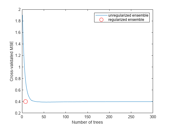
Figure contains an axes object. The axes object with xlabel Number of trees, ylabel Cross-validated MSE contains 2 objects of type line. One or more of the lines displays its values using only markers These objects represent unregularized ensemble, regularized ensemble.

新しいアンサンブルでは、大幅に少ないツリーを使用しながらも、損失を低く抑えています。

参考

アンサンブルの正則化

アンサンブル回帰の正則化

参考

トピック