Use Low Frequency Response Magnitude in Closed-Loop PID Autotuner

R2026b

This example shows how to use optional inputs in the Closed-Loop PID Autotuner block to reduce tuning time and increase the upper bound of achievable bandwidth.

Voltage-Mode Controlled Boost Converter

In this example, a voltage-mode boost converter is modeled in Simulink using Simscape™ Electrical™ components. The parameters of these components are based on [1].

mdl = "scdboostconverterPIDTuningMod";
open_system(mdl)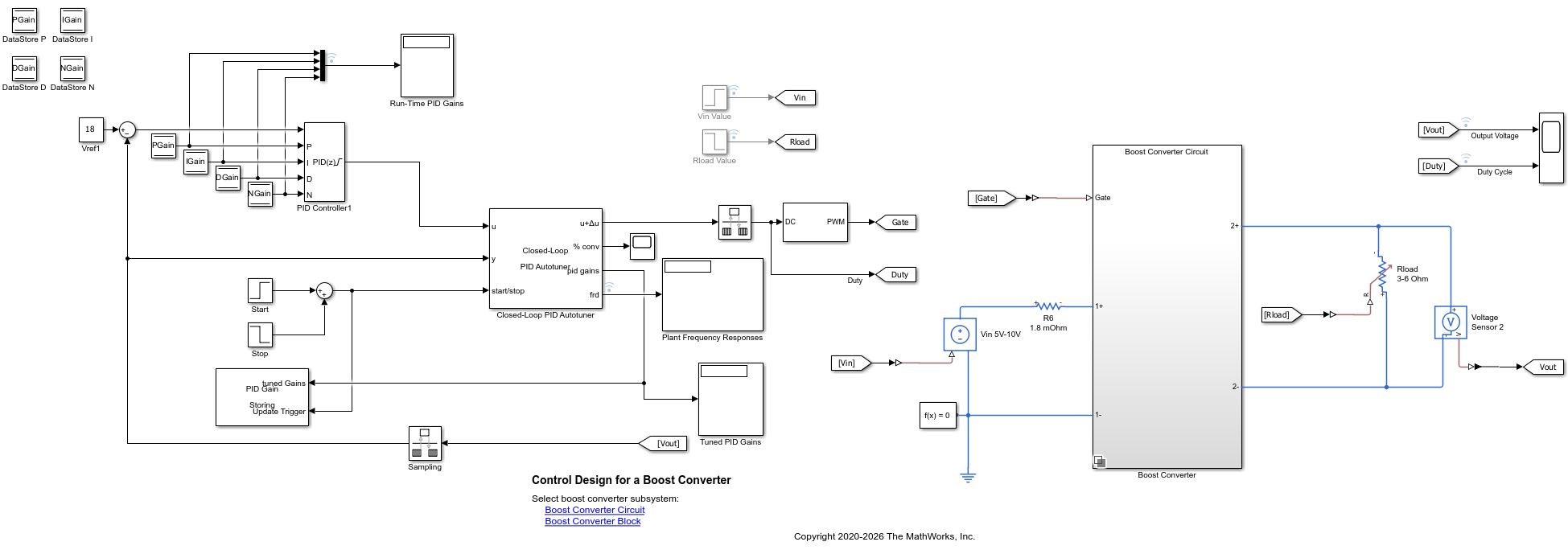

A boost converter circuit converts a DC voltage to another, typically higher, DC voltage by controlled chopping or switching of the source voltage. In this model, a MOSFET driven by a pulse-width modulation (PWM) signal is used for switching. A digital PID controller adjusts the PWM duty cycle to maintain the load voltage at its reference .

At the nominal operating point, the load voltage is 18 volts and the duty cycle is about 0.74. The duty cycle can vary from 0.1 to 0.85 during boost converter operation.

The existing PID controller has gains of $P$ = 0.02, $I$ = 160, $D$ = 0.00005, and $N$ = 20000. These gains are stored in a Data Store Memory block and provided externally to the PID Controller block. Having external gain input ports allows you to change the values after new gains are computed by the Closed-Loop PID Autotuner block.

Autotuner Block Configuration

The Closed-Loop PID Autotuner block is configured with the following settings.

On the Tuning tab, there are two main tuning settings.

• Target bandwidth: Determines how fast you want the controller to respond. In this example, use 10000 rad/sec is chosen, which is typical for a boost converter.

• Target phase margin: Determines how robust you want the controller to be. In this example, the default value of 60 degrees is chosen.

On the Experiment tab, there are three main experiment settings.

• Plant Type: Specifies whether the plant is asymptotically stable or integrating. In this example, the boost converter plant is stable.

• Plant Sign: Specifies whether the plant has a positive or negative sign. The plant sign is positive if a positive change in the plant input at the nominal operating point results in a positive change in the plant output when the plant reaches a new steady state. Otherwise, the plant sign is negative. If a plant is stable, plant sign is equivalent to the sign of its DC gain. If a plant is integrating, the plant sign is positive or negative if the plant output keeps increasing or decreasing, respectively. In this example, the boost converter plant has a positive plant sign.

• Signal Amplitudes: Specifies amplitudes of the injected signal. In this example, 0.03 is chosen for all five frequencies of the perturbation signal to ensure the plant is properly excited within the saturation limit. If the excitation amplitude is too large, the boost converter operates in discontinuous-current mode. If the input amplitude is too small, the sinusoidal signals are indistinguishable from ripples in the power electronics circuits. Both situations produce inaccurate frequency response estimation results.

Simulate Autotuner Block in Normal Mode

Simulation of the boost converter plant usually takes a few minutes because of the fast sample time of the PWM generator. Vout is the plant output and Duty Cycle is the plant input.

% Configure model for baseline
set_param(mdl+"/Closed-Loop PID Autotuner","EstimateLowFrequencyResponsePoint","on")
set_param(mdl+"/Closed-Loop PID Autotuner","LowFrequencyResponsePoint","0")
set_param(mdl+"/Stop","Time","0.06")

% Simulate
sim(mdl)

baselineResults = logsout;

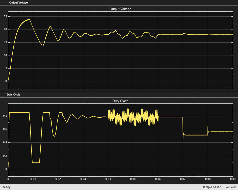
In this example, it takes the PID controller about 0.04 seconds to bring the boost converter to the nominal operating point of 18 volts. The initial transient contains strong oscillations, which indicates that the existing controller must be retuned.

At 0.04 seconds, the autotuning process starts. The experiment lasts 0.02 seconds, because the number of seconds it takes for the online frequency response estimation to converge is about 200 divided by the bandwidth.

When PID tuning stops at 0.06 seconds, the block calculates new gains, $P$ = 0.37, $I$ = 430, $D$ = 0.00009, and $N$ = 30000. The new gains are immediately written to the data store memory and sent to the external gain input ports of the PID Controller block, which overwrites the original gains.

The model has a line disturbance (Vin from 5V to 10V) and a load current disturbance (Load from 6A to 3A), which occur at 0.07 and 0.08 seconds, respectively. You can use these disturbances to examine controller performance.

Use Low Frequency Response Magnitude to Reduce Experiment Time

The Closed-Loop PID Autotuner block requires five frequency response points for use in the tuning algorithm: ${\omega }_c$*[1/10 1/3 1 3 10]. You can use the optional parameter, ${\omega }_c$/10 frequency response magnitude on the Experiment tab, to reduce the experiment time. You can obtain the value for this parameter different ways depending on what plant information you have. One common way to have this information is if you autotuned previously or used another frequency response based estimation method such as the Frequency Response Estimator block. The value for the magnitude at ${\omega }_c$/10 can also be derived with other known plant information such as the frequency response magnitude slope between ${\omega }_c$/10 and ${\omega }_c$/3. In this example the slope information is used to estimate the frequency response magnitude at ${\omega }_c$/10.

Use Plant Slope to Obtain Low Frequency Response Magnitude

As discussed previously, you can use information about the frequency response magnitude slope at lower frequencies to obtain the frequency response magnitude at ${\omega }_c$/10. Typically, this value is either 0 dB/decade or -20 dB/decade for a low pass filter like plant or plant with a pure integrator, respectively. For this system, it behaves like a pure integrator at lower frequencies resulting in a slope of -20 dB/decade. In order to determine the magnitude response at ${\omega }_c$/10, you can use the following equation with all values in dB:

$$y_2=y_{1+}m*{\log }_{10}\left(\frac{f_2}{f_1}\right)$$

The values of $f_2$ and $f_1$, ${\omega }_c$/3 and ${\omega }_c$/10, respectively, are known which reduces the above equation to:

$$y_2=y_1-m*0.5229$$

Using this equation, you obtain a $y_2$ magnitude, in dB, of 28.69 or 27.1844 in absolute units. You can use this value in the Closed-Loop PID Autotuner block for the ${\omega }_c$/10 frequency response magnitude and remove the need to estimate this point, which reduces the overall experiment time.

To enable this parameter, clear the Estimate frequency response at ${\omega }_c$/10 parameter.

set_param(mdl+"/Closed-Loop PID Autotuner", ...
    "EstimateLowFrequencyResponsePoint","off")

Specify the magnitude response at ${\omega }_c$/10 by setting the ${\omega }_c$/10 frequency response magnitude parameter.

set_param(mdl+"/Closed-Loop PID Autotuner", ...
    "LowFrequencyResponsePoint","27.1844")

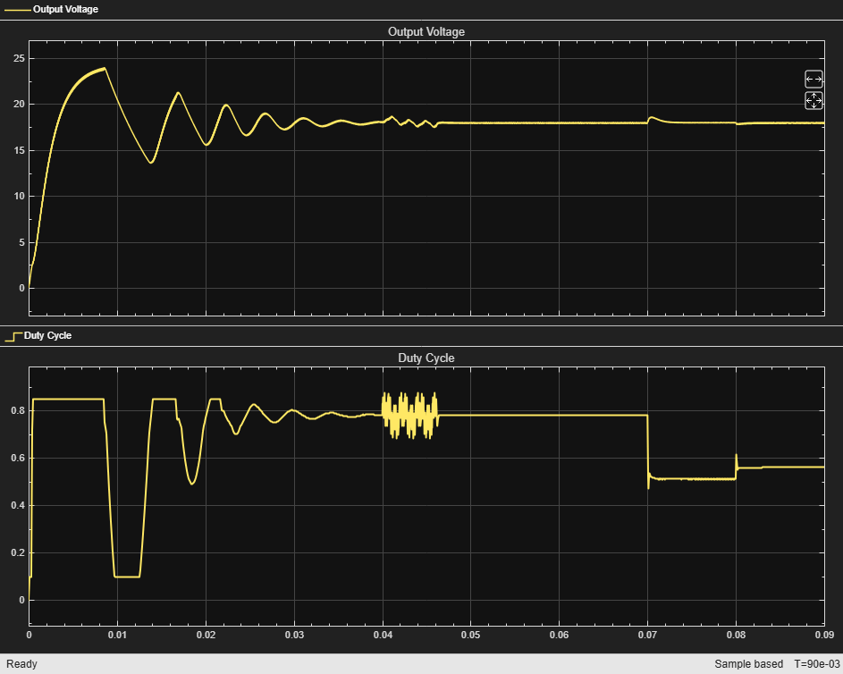
Previously, you needed an experiment length of 200/${\omega }_c$ seconds. Since you are specifying the magnitude at the lowest frequency point of ${\omega }_c$/10 the experiment length shortens to approximately 60/${\omega }_c$ seconds, which is 0.006 seconds for this example.

set_param(mdl+"/Stop","Time",'0.046')

Simulate Model in Normal Mode and Compare the Results

sim(mdl)

useSlopeResults = logsout;

Use DC Gain to Reduce Experiment Time

In the last section you used the slope information in order to estimate the low frequency point at bandwidth/10. You can, instead, use DC gain information for estimating the ${\omega }_c$/10 frequency point. You can use the below equation to obtain an estimate of the frequency response magnitude at ${\omega }_c$/10.

$$y_3=y_2+\left(y_2-y_1\right)\frac{{\log }_{10}\left(\frac{3}{10}\right)}{{\log }_{10}\left(\frac{N}{3}\right)}$$

In the above equation y1 is the DC gain value, y2 is the frequency response magnitude at ${\omega }_c$/3, $y_3$ is the frequency response magnitude at ${\omega }_c$/10 and $N$ is an integer number greater than 20. For systems with a DC gain value, the magnitude response levels off below some frequency. $N$ represents an estimate of where you expect this rolloff to start and can be adjusted as necessary to obtain better PID tuning results (${\omega }_{rolloff}={\omega }_c/N$). For this example you will use $N$ = 30.

You can calculate the DC gain value using the below equation for boost converters:

$$y_1=\frac{V_{out}}{1-Duty}$$

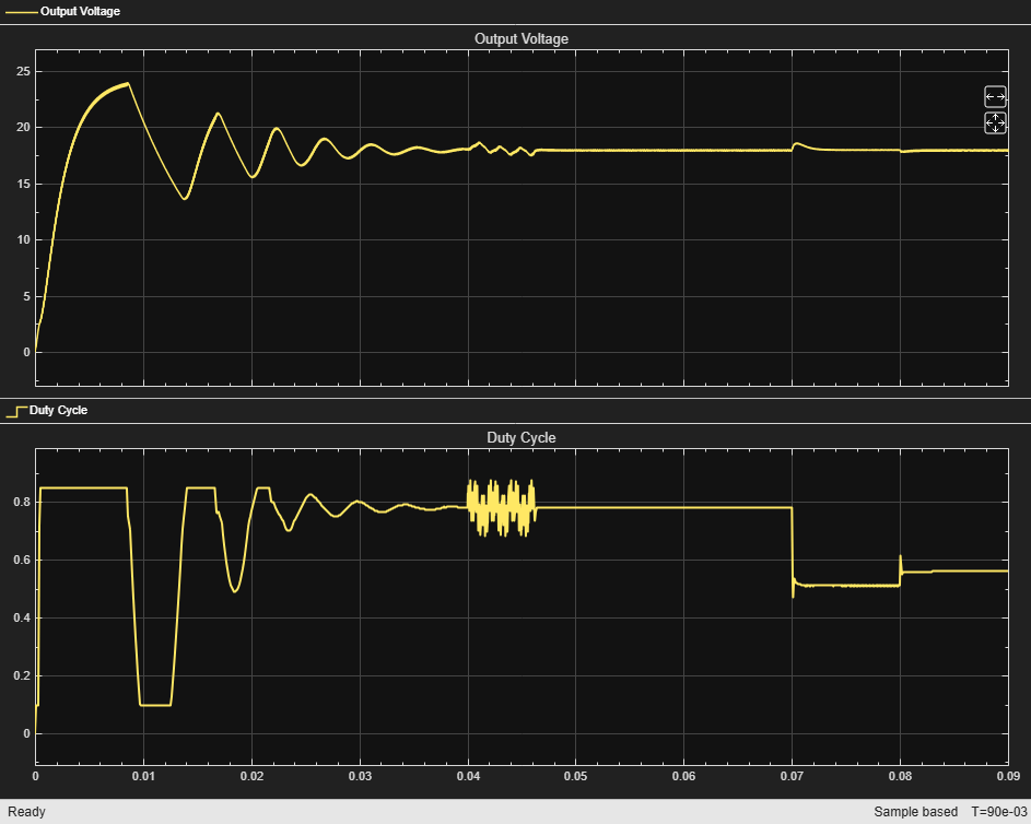
You can use the previous scope to estimate the output voltage, $V_{out}$, and the duty cycle, Duty, as 17.8 volts and 0.784, respectively. Using these values in the above equation results in a DC gain value of 82.41 or 38.32 dB. Using the value of 38.32 dB and an $N$ of 30 results in a $y_3$ magnitude of 29.28 dB or 29.1182 in absolute units. This value is close to the one you obtained previously using the slope instead of the DC gain value. You can use this value in the Closed-Loop PID Autotuner block and rerun the simulation to compare the results.

set_param(mdl+"/Closed-Loop PID Autotuner", ...
    "LowFrequencyResponsePoint","29.1182")
sim(mdl)

useDCgainResults = logsout;

Summary of Results

You can use the output voltage from the previous simulations to compare the responses using the three methods:

1. Estimate frequency response at ${\omega }_c$/10

2. Use slope information to obtain frequency response at ${\omega }_c$/10

3. Use DC gain information to obtain frequency response at ${\omega }_c$/10

idx1 = baselineResults{2}.Values.Time > 0.069;
idx2 = useSlopeResults{2}.Values.Time > 0.069;
idx3 = useDCgainResults{2}.Values.Time > 0.069;
figure
plot(baselineResults{2}.Values.Time(idx1), ...
    baselineResults{2}.Values.Data(idx1))
hold on
plot(useSlopeResults{2}.Values.Time(idx2), ...
    useSlopeResults{2}.Values.Data(idx2))
plot(useDCgainResults{2}.Values.Time(idx3), ...
    useDCgainResults{2}.Values.Data(idx3))
hold off
grid
xlabel("Time (sec)")
ylabel("Output Voltage (V)")
legend("baseline","slope","DC gain")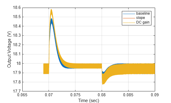

The results from the three simulations are similar.

Use High Frequency Response Magnitude to Increase Achievable Bandwidth

Similar to how specifying the low frequency response magnitude reduces the experiment time, you can specify the high frequency response magnitude, ${\omega }_c$*10, to increase the achievable bandwidth. Normally, you are limited to a highest achievable bandwidth of 0.3/$T_s$. However, specifying this high frequency response magnitude point allows for an achievable bandwidth of 1/$T_s$ or about 3 times higher. While not discussed in this example, you can use the same approach for the high frequency, ${\omega }_c$*10, response point.

References

[1] Lee, S. W. "Practical Feedback Loop Analysis for Voltage-Mode Boost Converter." Application Report No. SLVA633. Texas Instruments. January 2014. www.ti.com/lit/an/slva633/slva633.pdf