このページの内容は最新ではありません。最新版の英語を参照するには、ここをクリックします。

単側波帯振幅変調

この例では、ヒルベルト変換を使用して信号の単側波帯 (SSB) 振幅変調 (AM) を実行する方法を説明します。単側波帯 AM 信号の帯域幅は、通常の AM 信号の帯域幅より狭くなります。

関数 sinc を使用してシミュレートされた広帯域信号のサンプルを 512 個生成します。$$\pi /4$$ ラジアン/サンプルの帯域幅を指定します。

N = 512;
n = 0:N-1;

bw = 1/4;
x = sinc((n-N/2)*bw);

S/N 比が 20 dB となるホワイト ガウス ノイズを付加します。再現可能な結果が必要な場合は、乱数発生器をリセットします。関数 periodogram を使用して信号のパワー スペクトル密度 (PSD) を推定します。

rng default

SNR = 20;
noise = randn(size(x))*std(x)/db2mag(SNR);
x = x + noise;

periodogram(x)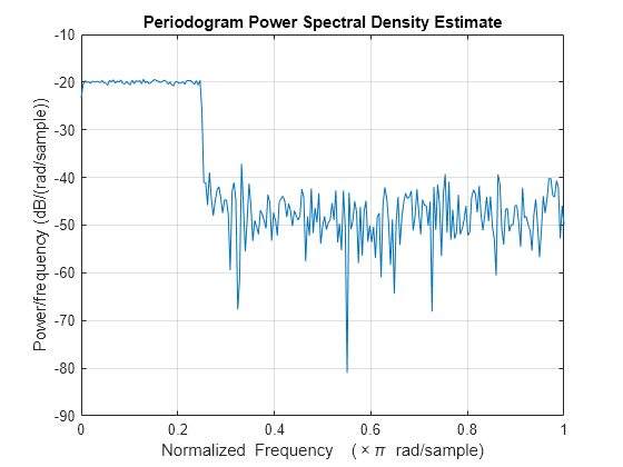

搬送周波数 $${\omega }_c=\pi /2$$ の余弦を使用して信号の振幅変調を行います。変調された信号のパワーが元の信号のパワーと等しくなるように $$\sqrt{2}$$ で乗算します。PSD を推定します。

wc = pi/2;

x1 = x.*cos(wc*n)*sqrt(2);

periodogram(x1)
legend('Modulated')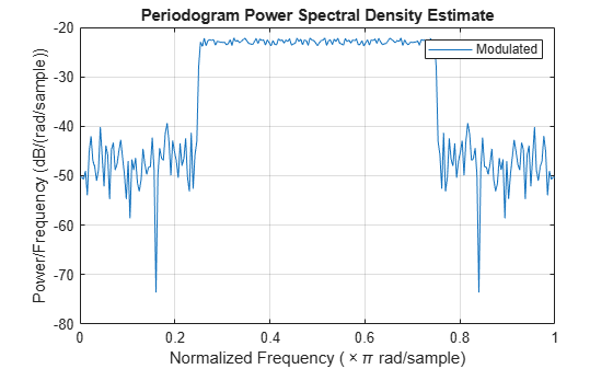

SSB 振幅変調では信号の帯域幅が半減します。SSB 振幅変調を実行するには、最初に信号のヒルベルト変換を計算しなければなりません。続いて、同じ搬送周波数 $${\omega }_c$$ を持つ正弦を使用して、前と同様に信号の振幅変調を行い、それを前の信号に付加します。

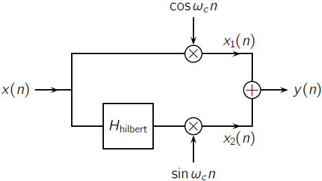
関数 designfilt を使用してヒルベルト変換器を設計します。フィルター次数 64 と遷移幅 0.1 を指定します。信号をフィルター処理します。

Hhilbert = designfilt('hilbertfir','FilterOrder',64, ...
    'TransitionWidth',0.1);

xh = filter(Hhilbert,x);

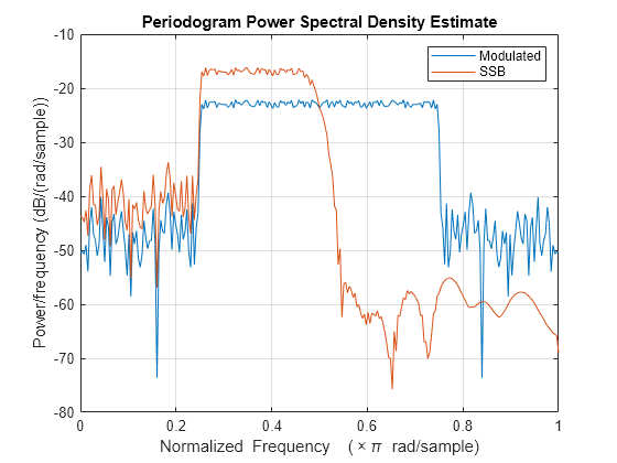
関数 grpdelay を使用して、フィルターによって生じる遅延 gd を測定します。フィルター処理した信号の最初の gd 点を破棄し、末尾をゼロでパディングすることで遅延を補正します。結果を振幅変調して元の信号に付加します。PSD を比較します。

gd = mean(grpdelay(Hhilbert));
xh = xh(gd+1:end);
eh = zeros(size(x));
eh(1:length(xh)) = xh;

x2 = eh.*sin(wc*n)*sqrt(2);

y = x1+x2;

periodogram([x1;y]')
legend('Modulated','SSB')

信号をダウンコンバートし、PSD を推定します。

ym = y.*cos(wc*n)*sqrt(2);

periodogram(ym)
legend('Downconverted')

変調された信号をローパス フィルター処理し、元の信号を復元します。カットオフ周波数 $$\pi /2$$ の 64 次 FIR ローパス フィルターを指定します。フィルターによって生じた遅延を補正します。

d = designfilt('lowpassfir','FilterOrder',64, ...
    'CutoffFrequency',0.5);
dem = filter(d,ym);

gd = mean(grpdelay(d));
dem = dem(gd+1:end);

dm = zeros(size(x));
dm(1:length(dem)) = dem;

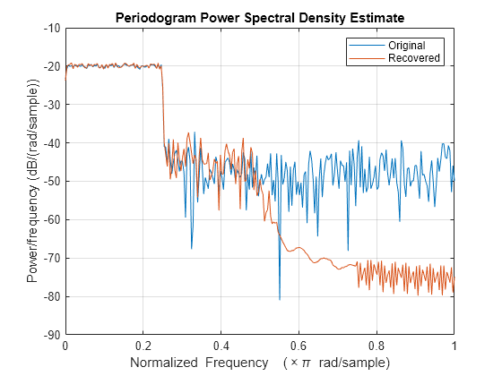
フィルター処理された信号の PSD を推定し、元の信号の PSD と比較します。

periodogram([x;dm]')
legend('Original','Recovered')

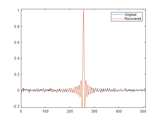
関数 snr を使用して 2 つの信号の S/N 比を比較します。時間領域に 2 つの信号をプロットします。

snrOrig = snr(x,noise)

snrOrig = 20.0259

snrRecv = snr(dm,noise)

snrRecv = 20.1373

plot(n,[x;dm]')
legend('Original','Recovered')
axis tight

参考文献

Buck, John R., Michael M. Daniel, and Andrew C. Singer. Computer Explorations in Signals and Systems Using MATLAB. 2nd Edition. Upper Saddle River, NJ: Prentice Hall, 2002.

参考

designfilt | periodogram | snr