h2syn
Compute H2 optimal controller
Syntax
Description
[
computes a stabilizing H2-optimal controller
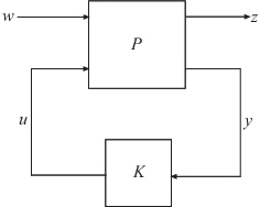
K,CL,gamma] = h2syn(P,nmeas,ncont)K for the plant P. The plant has a partitioned
form
where:
w represents the disturbance inputs.
u represents the control inputs.
z represents the error outputs to be kept small.
y represents the measurement outputs provided to the controller.
nmeas and ncont are the number of signals in
y and u, respectively. y and
u are the last outputs and inputs of P,
respectively. h2syn returns a controller K that
stabilizes P and has the same number of states. The closed-loop system
CL = lft(P,K) achieves the performance level
gamma, which is the H2 norm
of CL (see norm).
Examples
Stabilize a 5-by-4 unstable plant with three states, two measurement signals, and one control signal.
In practice, P is an augmented plant that you have constructed by combining a model of the system to control with appropriate weighting functions. For this example, use the following model.
A = [5    6    -6
     6    0     5
    -6    5     4];
B = [0     4     0     0
     1     1    -2    -2
     4     0     0    -3];
C = [-6     0     8
     0     5     0
    -2     1    -4
     4    -6    -5
     0   -15     7];
D = [0     0     0     0
     0     0     0     1
     0     0     0     0
     0     0     3     6
     8     0    -7     0];
P = ss(A,B,C,D);
Confirm that P is unstable by examining its poles, some of which lie in the right half-plane.
pole(P)
ans = 3×1

   -8.5648
    6.8612
   10.7036
Design the stabilizing controller. h2syn assumes that the nmeas measurement signals and the ncont control signals are the last outputs and last inputs of P, respectively.
nmeas = 2;
ncont = 1;
[K,CL,gamma] = h2syn(P,nmeas,ncont);
Examine the closed-loop system to confirm that the controller K stabilizes the plant.
pole(CL)
ans = 6×1 complex

 -31.6236 + 0.0000i
 -12.6460 + 3.8045i
 -12.6460 - 3.8045i
  -9.6073 + 0.0000i
  -9.2393 + 0.0000i
  -8.6939 + 0.0000i
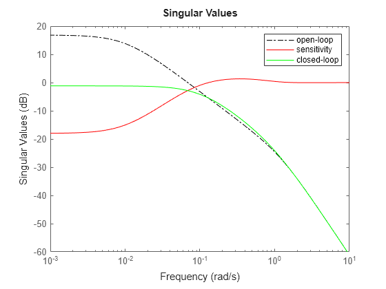
Shape the singular value plots of the sensitivity and complementary sensitivity .
To do so, find a stabilizing controller K that minimizes the norm of:

Assume the following plant and weights:
Using those values, construct the augmented plant P, as illustrated in the mixsyn reference page.
s = zpk('s');
G = 10*(s-1)/(s+1)^2;
G.u = 'u2';
G.y = 'y';

W1 = 0.1/(100*s+1);
W1.u = 'y2';
W1.y = 'y11';

W2 = tf(0.1);
W2.u = 'u2';
W2.y = 'y12';

S = sumblk('y2 = u1 - y');

P = connect(G,S,W1,W2,{'u1','u2'},{'y11','y12','y2'});
Use h2syn to generate the controller. This system has one measurement signal and one control signal, which are the last output and input of P, respectively.
[K,CL,gamma] = h2syn(P,1,1);
Examine the resulting loop shapes.
L = G*K;
S = inv(1+L);
T = 1-S;
sigmaplot(L,'k-.',S,'r',T,'g')
legend('open-loop','sensitivity','closed-loop')
Input Arguments
Output Arguments
Closed-loop transfer function, returned as a state-space (ss) model
object or []. The closed-loop transfer function is CL =
lft(P,K) as in the following diagram.
Additional synthesis data, returned as a structure. info has
the following fields.
| Field | Description |
|---|---|
X | Solution of state-feedback Riccati equation, returned as a matrix. |
Y | Solution of observer Riccati equation, returned as a matrix. |
Ku | State feedback gain of in the observer form of controller
|
Lx,Lu | Observer gains of the observer form of controller
|
Preg | Regularized plant used for |
NORMS | Costs for the synthesized controller, returned in a vector of the
form
These quantities are related by |
KFI | Full-information state-feedback gain, returned as a matrix. The
full-information problem assumes full knowledge of the state
For more information, see section 14.8 of [1]. |
GFI | Full-information closed-loop transfer from w to
z with the controller KFI, returned as a
state-space (ss) model. The
H2 norm of GFI is
FI. |
HAMX,HAMY | X Hamiltonian matrix (state feedback) and Y Hamiltonian matrix (Kalman
filter). These values are provided for reference, but h2syn
does not use them to compute the Riccati solutions. Instead,
h2syn uses the implicit solvers
icare and idare. |
Tips
h2syngives you state-feedback gain and observer gains that you can use to express the controller in observer form. The observer form of the controllerKis:Here, the innovation term e is:
h2synreturns the state-feedback gain Ku and the observer gains Lx and Lu as fields in theinfooutput argument.You can use this form of the controller for gain scheduling in Simulink®. To do so, tabulate the plant matrices and the controller gain matrices as a function of the scheduling variables using the Matrix Interpolation (Simulink) block. Then, use the observer form of the controller to update the controller variables as the scheduling variables change.
Do not choose weighting functions with poles very close to s = 0 (z = 1 for discrete-time systems). For instance, although it might seem sensible to choose W = 1/s to enforce zero steady-state error, doing so introduces an unstable pole that cannot be stabilized, causing synthesis to fail. Instead, choose W = 1/(s + δ). The value δ must be small but not very small compared to system dynamics. For instance, for best numeric results, if your target crossover frequency is around 1 rad/s, choose δ = 0.0001 or 0.001. Similarly, in discrete time, choose sample times such that system and weighting dynamics are not more than a decade or two below the Nyquist frequency.
Algorithms
h2syn uses the methods described in Chapter 14 of [1].
References
[1] Zhou, K., Doyle, J., Glover, K, Robust and Optimal Control. Upper Saddle River, NJ: Prentice Hall, 1996.
Version History
Introduced before R2006a