modelDiscrimination

Compute AUROC and ROC data

Syntax

DiscMeasure = modelDiscrimination(pdModel,data)

[DiscMeasure,DiscData] = modelDiscrimination(___,Name,Value)

Description

DiscMeasure = modelDiscrimination(pdModel,data) computes the area under the receiver operating characteristic curve (AUROC). modelDiscrimination supports segmentation and comparison against a reference model.

[DiscMeasure,DiscData] = modelDiscrimination(___,Name,Value) specifies options using one or more name-value pair arguments in addition to the input arguments in the previous syntax.

Examples

Generate AUROC and ROC for Logistic Lifetime PD Model

This example shows how to use fitLifetimePDModel to fit data with a Logistic model and then generate the area under the receiver operating characteristic curve (AUROC) and ROC curve.

Load Data

Load the credit portfolio data.

load RetailCreditPanelData.mat
disp(head(data))

    ID    ScoreGroup    YOB    Default    Year
    __    __________    ___    _______    ____

    1      Low Risk      1        0       1997
    1      Low Risk      2        0       1998
    1      Low Risk      3        0       1999
    1      Low Risk      4        0       2000
    1      Low Risk      5        0       2001
    1      Low Risk      6        0       2002
    1      Low Risk      7        0       2003
    1      Low Risk      8        0       2004

disp(head(dataMacro))

    Year     GDP     Market
    ____    _____    ______

    1997     2.72      7.61
    1998     3.57     26.24
    1999     2.86      18.1
    2000     2.43      3.19
    2001     1.26    -10.51
    2002    -0.59    -22.95
    2003     0.63      2.78
    2004     1.85      9.48

Join the two data components into a single data set.

data = join(data,dataMacro);
disp(head(data))

    ID    ScoreGroup    YOB    Default    Year     GDP     Market
    __    __________    ___    _______    ____    _____    ______

    1      Low Risk      1        0       1997     2.72      7.61
    1      Low Risk      2        0       1998     3.57     26.24
    1      Low Risk      3        0       1999     2.86      18.1
    1      Low Risk      4        0       2000     2.43      3.19
    1      Low Risk      5        0       2001     1.26    -10.51
    1      Low Risk      6        0       2002    -0.59    -22.95
    1      Low Risk      7        0       2003     0.63      2.78
    1      Low Risk      8        0       2004     1.85      9.48

Partition Data

Separate the data into training and test partitions.

nIDs = max(data.ID);
uniqueIDs = unique(data.ID);

rng('default'); % for reproducibility
c = cvpartition(nIDs,'HoldOut',0.4);

TrainIDInd = training(c);
TestIDInd = test(c);

TrainDataInd = ismember(data.ID,uniqueIDs(TrainIDInd));
TestDataInd = ismember(data.ID,uniqueIDs(TestIDInd));

Create a Logistic Lifetime PD Model

Use fitLifetimePDModel to create a Logistic model.

pdModel = fitLifetimePDModel(data(TrainDataInd,:),"Logistic",...
    'AgeVar','YOB',...
    'IDVar','ID',...
    'LoanVars','ScoreGroup',...
    'MacroVars',{'GDP','Market'},...
    'ResponseVar','Default');
 disp(pdModel)

  Logistic with properties:

            ModelID: "Logistic"
        Description: ""
    UnderlyingModel: [1×1 classreg.regr.CompactGeneralizedLinearModel]
              IDVar: "ID"
             AgeVar: "YOB"
           LoanVars: "ScoreGroup"
          MacroVars: ["GDP"    "Market"]
        ResponseVar: "Default"
         WeightsVar: ""
       TimeInterval: 1

Display the underlying model.

pdModel.UnderlyingModel 

ans = 
Compact generalized linear regression model:
    logit(Default) ~ 1 + ScoreGroup + YOB + GDP + Market
    Distribution = Binomial

Estimated Coefficients:
                               Estimate        SE         tStat       pValue   
                              __________    _________    _______    ___________

    (Intercept)                  -2.7422      0.10136    -27.054     3.408e-161
    ScoreGroup_Medium Risk      -0.68968     0.037286    -18.497     2.1894e-76
    ScoreGroup_Low Risk          -1.2587     0.045451    -27.693    8.4736e-169
    YOB                         -0.30894     0.013587    -22.738    1.8738e-114
    GDP                         -0.11111     0.039673    -2.8006      0.0051008
    Market                    -0.0083659    0.0028358    -2.9502      0.0031761


388097 observations, 388091 error degrees of freedom
Dispersion: 1
Chi^2-statistic vs. constant model: 1.85e+03, p-value = 0

pdModel.UnderlyingModel.Coefficients

ans=6×4 table
                               Estimate        SE         tStat       pValue   
                              __________    _________    _______    ___________

    (Intercept)                  -2.7422      0.10136    -27.054     3.408e-161
    ScoreGroup_Medium Risk      -0.68968     0.037286    -18.497     2.1894e-76
    ScoreGroup_Low Risk          -1.2587     0.045451    -27.693    8.4736e-169
    YOB                         -0.30894     0.013587    -22.738    1.8738e-114
    GDP                         -0.11111     0.039673    -2.8006      0.0051008
    Market                    -0.0083659    0.0028358    -2.9502      0.0031761

Model Discrimination to Generate AUROC and ROC

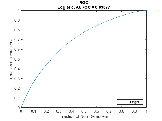
Model "discrimination" measures how effectively a model ranks customers by risk. You can use the AUROC and ROC outputs to determine whether customers with higher predicted PDs actually have higher risk in the observed data.

DataSetChoice = "Training";
if DataSetChoice=="Training"
    Ind = TrainDataInd;
 else
    Ind = TestDataInd;
 end

DiscMeasure = modelDiscrimination(pdModel,data(TrainDataInd,:),'ShowDetails',true,'DataID',DataSetChoice);
disp(DiscMeasure)

                           AUROC      Segment      SegmentCount    WeightedCount
                          _______    __________    ____________    _____________

    Logistic, Training    0.69377    "all_data"     3.881e+05        3.881e+05  

Visualize the ROC for the Logistic model using modelDiscriminationPlot.

modelDiscriminationPlot(pdModel,data(TrainDataInd,:)); 

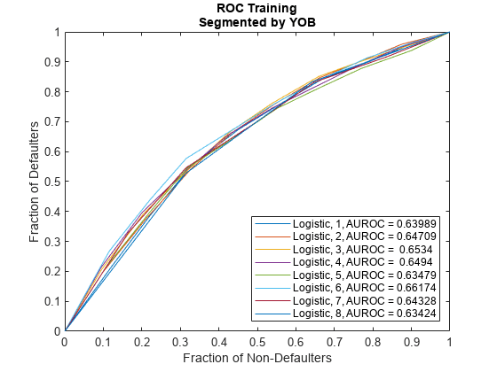
Data can be segmented to get the AUROC per segment and the corresponding ROC data.

SegmentVar = "YOB";
DiscMeasure = modelDiscrimination(pdModel,data(Ind,:),'ShowDetails',true,'SegmentBy',SegmentVar,'DataID',DataSetChoice);
disp(DiscMeasure)

                                  AUROC     Segment    SegmentCount    WeightedCount
                                 _______    _______    ____________    _____________

    Logistic, YOB=1, Training    0.63989       1          58092            58092    
    Logistic, YOB=2, Training    0.64709       2          56723            56723    
    Logistic, YOB=3, Training     0.6534       3          55524            55524    
    Logistic, YOB=4, Training     0.6494       4          54650            54650    
    Logistic, YOB=5, Training    0.63479       5          53770            53770    
    Logistic, YOB=6, Training    0.66174       6          53186            53186    
    Logistic, YOB=7, Training    0.64328       7          36959            36959    
    Logistic, YOB=8, Training    0.63424       8          19193            19193    

Visualize the ROC segmented by YOB, ScoreGroup, or Year using modelDiscriminationPlot.

modelDiscriminationPlot(pdModel,data(Ind,:),'SegmentBy',SegmentVar,'DataID',DataSetChoice);

Input Arguments

pdModel — Probability of default model

Logistic object | Probit object | Cox object | customLifetimePDModel object

Probability of default model, specified as a Logistic, Probit, or Cox object previously created using fitLifetimePDModel. Alternatively, you can create a custom probability of default model using customLifetimePDModel.

Note

The 'ModelID' property of the pdModel object is used as the identifier or tag for pdModel.

Data Types: object

data — Data

table

Data, specified as a NumRows-by-NumCols table with projected predictor values to make lifetime predictions. The predictor names and data types must be consistent with the underlying model.

Data Types: table

Name-Value Arguments

Specify optional pairs of arguments as Name1=Value1,...,NameN=ValueN, where Name is the argument name and Value is the corresponding value. Name-value arguments must appear after other arguments, but the order of the pairs does not matter.

Before R2021a, use commas to separate each name and value, and enclose Name in quotes.

Example: [PerfMeasure,PerfData] = modelDiscrimination(pdModel,data(Ind,:),'DataID',"DataSetChoice")

DataID — Data set identifier

"" (default) | character vector | string

Data set identifier, specified as the comma-separated pair consisting of 'DataID' and a character vector or string.

Data Types: char | string

SegmentBy — Name of column in data input used to segment data set

"" (default) | character vector | string

Name of a column in the data input, not necessarily a model variable, to be used to segment the data set, specified as the comma-separated pair consisting of 'SegmentBy' and a character vector or string.

One AUROC value is reported for each segment and the corresponding ROC data for each segment is returned in the PerfData optional output.

Data Types: char | string

ShowDetails — Indicates if output includes columns showing segment value, segment count, and weighted count

false (default) | logical

Since R2022a

Indicates if the output includes columns showing segment value, segment count, and weighted count, specified as the comma-separated pair consisting of 'ShowDetails' and a scalar logical.

Data Types: logical

ReferencePD — Conditional PD values predicted for data by reference model

[ ] (default) | numeric vector

Conditional PD values predicted for data by the reference model, specified as the comma-separated pair consisting of 'ReferencePD' and a NumRows-by-1 numeric vector. The modelDiscrimination output information is reported for both the pdModel object and the reference model.

Data Types: double

ReferenceID — Identifier for reference model

'Reference' (default) | character vector | string

Identifier for the reference model, specified as the comma-separated pair consisting of 'ReferenceID' and a character vector or string. 'ReferenceID' is used in the modelDiscrimination output for reporting purposes.

Data Types: char | string

Output Arguments

DiscMeasure — AUROC information for each model and each segment

table

AUROC information for each model and each segment, returned as a table. DiscMeasure has a single column named 'AUROC' and the number of rows depends on the number of segments and whether you use a ReferenceID for a reference model and ReferencePD for reference data. The row names of DiscMeasure report the model IDs, segment, and data ID. If the optional ShowDetails name-value argument is true, the DiscMeasure output displays Segment, SegmentCount, and WeightedCount columns.

Note

If you do not specify SegmentBy and use ShowDetails to request the segment details, the two columns are added and show the Segment column as "all_data" and the sample size (minus missing values) for the SegmentCount column.

DiscData — ROC data for each model and each segment

table

ROC data for each model and each segment, returned as a table. There are three columns for the ROC data, with column names 'X', 'Y', and 'T', where the first two are the X and Y coordinates of the ROC curve, and T contains the corresponding thresholds.

If you use SegmentBy, the function stacks the ROC data for all segments and DiscData has a column with the segmentation values to indicate where each segment starts and ends.

If reference model data is given using ReferenceID and ReferencePD, the DiscData outputs for the main and reference models are stacked, with an extra column 'ModelID' indicating where each model starts and ends.

More About

Model Discrimination

Model discrimination measures the risk ranking.

Higher-risk loans should get higher predicted probability of default (PD) than lower-risk loans. The modelDiscrimination function computes the Area Under the Receiver Operator Characteristic curve (AUROC), sometimes called simply the Area Under the Curve (AUC). This metric is between 0 and 1 and higher values indicate better discrimination.

For more information about the Receiver Operator Characteristic (ROC) curve, see Model Discrimination and ROC Curve and Performance Metrics.

References

[1] Baesens, Bart, Daniel Roesch, and Harald Scheule. Credit Risk Analytics: Measurement Techniques, Applications, and Examples in SAS. Wiley, 2016.

[2] Bellini, Tiziano. IFRS 9 and CECL Credit Risk Modelling and Validation: A Practical Guide with Examples Worked in R and SAS. San Diego, CA: Elsevier, 2019.

[3] Breeden, Joseph. Living with CECL: The Modeling Dictionary. Santa Fe, NM: Prescient Models LLC, 2018.

[4] Roesch, Daniel and Harald Scheule. Deep Credit Risk: Machine Learning with Python. Independently published, 2020.

Version History

Introduced in R2020b

R2023b: Support for WeightedCount column in DiscMeasure output

The DiscMeasure output supports an additional column for WeightedCount.

R2022b: Support for customLifetimePDModel model

The pdModel input supports an option for a customLifetimePDModel model object that you can create using customLifetimePDModel.

R2022a: Additional option for ShowDetails

There is an additional name-value pair for ShowDetails to indicate if the DiscMeasure output includes columns for Segment value and the SegmentCount.