Compare Probability of Default Using Through-the-Cycle and Point-in-Time Models
This example shows how to work with consumer credit panel data to create through-the-cycle (TTC) and point-in-time (PIT) models and compare their respective probabilities of default (PD).
The PD of an obligor is a fundamental risk parameter in credit risk analysis. The PD of an obligor depends on customer-specific risk factors as well as macroeconomic risk factors. Because they incorporate macroeconomic conditions differently, TTC and PIT models produce different PD estimates.
A TTC credit risk measure primarily reflects the credit risk trend of a customer over the long term. Transient, short-term changes in credit risk that are likely to be reversed with the passage of time get smoothed out. The predominant features of TTC credit risk measures are their high degree of stability over the credit cycle and the smoothness of change over time.
A PIT credit risk measure utilizes all available and pertinent information as of a given date to estimate the PD of a customer over a given time horizon. The information set includes not just expectations about the credit risk trend of a customer over the long term but also geographic, macroeconomic, and macro-credit trends.
Previously, according to the Basel II rules, regulators called for the use of TTC PDs, losses given default (LGDs), and exposures at default (EADs). However, with to the new IFRS9 and proposed CECL accounting standards, regulators now require institutions to use PIT projections of PDs, LGDs, and EADs. By accounting for the current state of the credit cycle, PIT measures closely track the variations in default and loss rates over time.
Load Panel Data
The main data set in this example (data) contains the following variables:
ID —Loan identifier.ScoreGroup —Credit score at the beginning of the loan, discretized into three groups:High Risk,Medium Risk, andLow Risk.YOB —Years on books.Default —Default indicator. This is the response variable.Year —Calendar year.
The data also includes a small data set (dataMacro) with macroeconomic data for the corresponding calendar years:
Year —Calendar year.GDP —Gross domestic product growth (year over year).Market —Market return (year over year).
The variables YOB, Year, GDP, and Market are observed at the end of the corresponding calendar year. ScoreGroup is a discretization of the original credit score when the loan started. A value of 1 for Default means that the loan defaulted in the corresponding calendar year.
This example uses simulated data, but you can apply the same approach to real data sets.
Load the data and view the first 10 rows of the table. The panel data is stacked and the observations for the same ID are stored in contiguous rows, creating a tall, thin table. The panel is unbalanced because not all IDs have the same number of observations.
load RetailCreditPanelData.mat
disp(head(data,10));
ID ScoreGroup YOB Default Year
__ ___________ ___ _______ ____
1 Low Risk 1 0 1997
1 Low Risk 2 0 1998
1 Low Risk 3 0 1999
1 Low Risk 4 0 2000
1 Low Risk 5 0 2001
1 Low Risk 6 0 2002
1 Low Risk 7 0 2003
1 Low Risk 8 0 2004
2 Medium Risk 1 0 1997
2 Medium Risk 2 0 1998
nRows = height(data);
UniqueIDs = unique(data.ID);
nIDs = length(UniqueIDs);
fprintf('Total number of IDs: %d\n',nIDs)
Total number of IDs: 96820
fprintf('Total number of rows: %d\n',nRows)Total number of rows: 646724
Default Rates by Year
Use Year as a grouping variable to compute the observed default rate for each year. Use the groupsummary function to compute the mean of the Default variable, grouping by the Year variable. Plot the results on a scatter plot which shows that the default rate goes down as the years increase.
DefaultPerYear = groupsummary(data,'Year','mean','Default');
NumYears = height(DefaultPerYear);
disp(DefaultPerYear)
    Year    GroupCount    mean_Default
    ____    __________    ____________

    1997      35214         0.018629
    1998      66716         0.013355
    1999      94639         0.012733
    2000      92891         0.011379
    2001      91140         0.010742
    2002      89847         0.010295
    2003      88449        0.0056417
    2004      87828        0.0032905
subplot(2,1,1)
scatter(DefaultPerYear.Year, DefaultPerYear.mean_Default*100,'*');
grid on
xlabel('Year')
ylabel('Default Rate (%)')
title('Default Rate per Year')
% Get IDs of the 1997, 1998, and 1999 cohorts
IDs1997 = data.ID(data.YOB==1&data.Year==1997);
IDs1998 = data.ID(data.YOB==1&data.Year==1998);
IDs1999 = data.ID(data.YOB==1&data.Year==1999);
% Get default rates for each cohort separately
ObsDefRate1997 = groupsummary(data(ismember(data.ID,IDs1997),:),...
    'YOB','mean','Default');

ObsDefRate1998 = groupsummary(data(ismember(data.ID,IDs1998),:),...
    'YOB','mean','Default');

ObsDefRate1999 = groupsummary(data(ismember(data.ID,IDs1999),:),...
    'YOB','mean','Default');
% Plot against the calendar year
Year = unique(data.Year);
subplot(2,1,2)
plot(Year,ObsDefRate1997.mean_Default*100,'-*')
hold on
plot(Year(2:end),ObsDefRate1998.mean_Default*100,'-*')
plot(Year(3:end),ObsDefRate1999.mean_Default*100,'-*')
hold off
title('Default Rate vs. Calendar Year')
xlabel('Calendar Year')
ylabel('Default Rate (%)')
legend('Cohort 97','Cohort 98','Cohort 99')
grid on
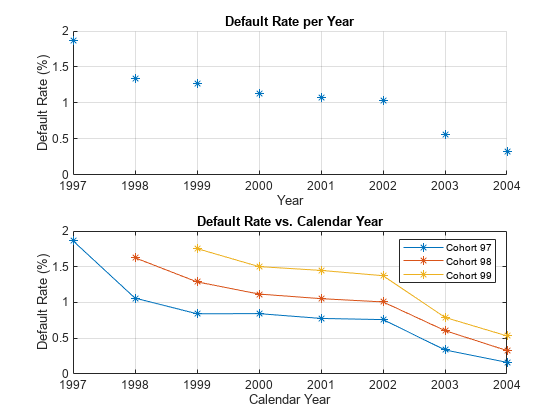
The plot shows that the default rate decreases over time. Notice in the plot that loans starting in the years 1997, 1998, and 1999 form three cohorts. No loan in the panel data starts after 1999. This is depicted in more detail in the "Years on Books Versus Calendar Years" section of the example on Stress Testing of Consumer Credit Default Probabilities Using Panel Data. The decreasing trend in this plot is explained by the fact that there are only three cohorts in the data and that the pattern for each cohort is decreasing.
TTC Model Using ScoreGroup and Years on Books
TTC models are largely unaffected by economic conditions. The first TTC model in this example uses only ScoreGroup and YOB as predictors of the default rate.
Generate training and testing data sets by splitting the existing data into training and testing data sets that are used for model creation and validation, respectively.
NumTraining = floor(0.6*nIDs);

rng('default');
TrainIDInd = randsample(nIDs,NumTraining);
TrainDataInd = ismember(data.ID,UniqueIDs(TrainIDInd));
TestDataInd = ~TrainDataInd;
Use the fitLifetimePDModel function to fit a Logistic model.
TTCModel = fitLifetimePDModel(data(TrainDataInd,:),'logistic',...
   'ModelID','TTC','IDVar','ID','AgeVar','YOB','LoanVars','ScoreGroup',...
   'ResponseVar','Default');
disp(TTCModel.Model)
Compact generalized linear regression model:
    logit(Default) ~ 1 + ScoreGroup + YOB
    Distribution = Binomial

Estimated Coefficients:
                              Estimate       SE        tStat       pValue
                              ________    ________    _______    ___________

    (Intercept)                -3.2453    0.033768    -96.106              0
    ScoreGroup_Medium Risk     -0.7058    0.037103    -19.023     1.1014e-80
    ScoreGroup_Low Risk        -1.2893    0.045635    -28.253    1.3076e-175
    YOB                       -0.22693    0.008437    -26.897    2.3578e-159


388018 observations, 388014 error degrees of freedom
Dispersion: 1
Chi^2-statistic vs. constant model: 1.83e+03, p-value = 0
Predict the PD for the training and testing data sets using predict.
data.TTCPD = zeros(height(data),1);

% Predict the in-sample
data.TTCPD(TrainDataInd) = predict(TTCModel,data(TrainDataInd,:));
% Predict the out-of-sample
data.TTCPD(TestDataInd) = predict(TTCModel,data(TestDataInd,:));
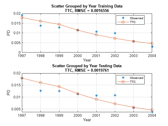
Visualize the in-sample fit and out-of-sample fit using modelCalibrationPlot.
figure;
subplot(2,1,1)
modelCalibrationPlot(TTCModel,data(TrainDataInd,:),'Year','DataID',"Training Data")
subplot(2,1,2)
modelCalibrationPlot(TTCModel,data(TestDataInd,:),'Year','DataID',"Testing Data")
PIT Model Using ScoreGroup, Years on Books, GDP, and Market Returns
PIT models vary with the economic cycle. The PIT model in this example uses ScoreGroup, YOB, GDP, and Market as predictors of the default rate. Use the fitLifetimePDModel function to fit a Logistic model.
% Add the GDP and Market returns columns to the original data

data = join(data, dataMacro);
disp(head(data,10))
ID ScoreGroup YOB Default Year TTCPD GDP Market
__ ___________ ___ _______ ____ _________ _____ ______
1 Low Risk 1 0 1997 0.0084797 2.72 7.61
1 Low Risk 2 0 1998 0.0067697 3.57 26.24
1 Low Risk 3 0 1999 0.0054027 2.86 18.1
1 Low Risk 4 0 2000 0.0043105 2.43 3.19
1 Low Risk 5 0 2001 0.0034384 1.26 -10.51
1 Low Risk 6 0 2002 0.0027422 -0.59 -22.95
1 Low Risk 7 0 2003 0.0021867 0.63 2.78
1 Low Risk 8 0 2004 0.0017435 1.85 9.48
2 Medium Risk 1 0 1997 0.015097 2.72 7.61
2 Medium Risk 2 0 1998 0.012069 3.57 26.24
PITModel = fitLifetimePDModel(data(TrainDataInd,:),'logistic',...
   'ModelID','PIT','IDVar','ID','AgeVar','YOB','LoanVars','ScoreGroup',...
   'MacroVars',{'GDP' 'Market'},'ResponseVar','Default');
disp(PITModel.Model)
Compact generalized linear regression model:
    logit(Default) ~ 1 + ScoreGroup + YOB + GDP + Market
    Distribution = Binomial

Estimated Coefficients:
                               Estimate        SE         tStat       pValue
                              __________    _________    _______    ___________

    (Intercept)                   -2.667      0.10146    -26.287    2.6919e-152
    ScoreGroup_Medium Risk      -0.70751     0.037108    -19.066     4.8223e-81
    ScoreGroup_Low Risk          -1.2895     0.045639    -28.253    1.2892e-175
    YOB                         -0.32082     0.013636    -23.528    2.0867e-122
    GDP                         -0.12295     0.039725     -3.095      0.0019681
    Market                    -0.0071812    0.0028298    -2.5377       0.011159


388018 observations, 388012 error degrees of freedom
Dispersion: 1
Chi^2-statistic vs. constant model: 1.97e+03, p-value = 0
Predict the PD for training and testing data sets using predict.
data.PITPD = zeros(height(data),1);

% Predict in-sample
data.PITPD(TrainDataInd) = predict(PITModel,data(TrainDataInd,:));
% Predict out-of-sample
data.PITPD(TestDataInd) = predict(PITModel,data(TestDataInd,:));
Visualize the in-sample fit and out-of-sample fit using modelCalibrationPlot.
figure;
subplot(2,1,1)
modelCalibrationPlot(PITModel,data(TrainDataInd,:),'Year','DataID',"Training Data")
subplot(2,1,2)
modelCalibrationPlot(PITModel,data(TestDataInd,:),'Year','DataID',"Testing Data")
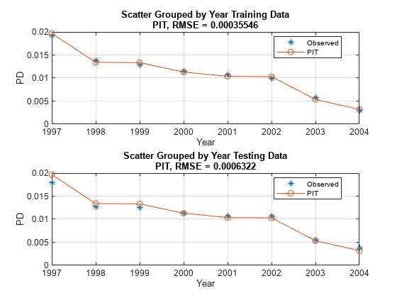
In the PIT model, as expected, the predictions match the observed default rates more closely than in the TTC model. Although this example uses simulated data, qualitatively, the same type of model improvement is expected when moving from TTC to PIT models for real world data, although the overall error might be larger than in this example. The PIT model fit is typically better than the TTC model fit and the predictions typically match the observed rates.
Calculate TTC PD Using the PIT Model
Another approach for calculating TTC PDs is to use the PIT model and then replace the GDP and Market returns with the respective average values. In this approach, you use the mean values over an entire economic cycle (or an even longer period) so that only baseline economic conditions influence the model, and any variability in default rates is due to other risk factors. You can also enter forecasted baseline values for the economy that are different from the mean observed for the most recent economic cycle. For example, using the median instead of the mean reduces the error.
You can also use this approach of calculating TTC PDs by using the PIT model as a tool for scenario analysis, however; this cannot be done in the first version of the TTC model. The added advantage of this approach is that you can use a single model for both the TTC and PIT predictions. This means that you need to validate and maintain only one model.
% Modify the data to replace the GDP and Market returns with the corresponding average values
data.GDP(:) = median(data.GDP);
data.Market = repmat(mean(data.Market), height(data), 1);
disp(head(data,10));
ID ScoreGroup YOB Default Year TTCPD GDP Market PITPD
__ ___________ ___ _______ ____ _________ ____ ______ _________
1 Low Risk 1 0 1997 0.0084797 1.85 3.2263 0.0093187
1 Low Risk 2 0 1998 0.0067697 1.85 3.2263 0.005349
1 Low Risk 3 0 1999 0.0054027 1.85 3.2263 0.0044938
1 Low Risk 4 0 2000 0.0043105 1.85 3.2263 0.0038285
1 Low Risk 5 0 2001 0.0034384 1.85 3.2263 0.0035402
1 Low Risk 6 0 2002 0.0027422 1.85 3.2263 0.0035259
1 Low Risk 7 0 2003 0.0021867 1.85 3.2263 0.0018336
1 Low Risk 8 0 2004 0.0017435 1.85 3.2263 0.0010921
2 Medium Risk 1 0 1997 0.015097 1.85 3.2263 0.016554
2 Medium Risk 2 0 1998 0.012069 1.85 3.2263 0.0095319
Predict the PD for training and testing data sets using predict.
data.TTCPD2 = zeros(height(data),1);

% Predict in-sample
data.TTCPD2(TrainDataInd) = predict(PITModel,data(TrainDataInd,:));
% Predict out-of-sample
data.TTCPD2(TestDataInd) = predict(PITModel,data(TestDataInd,:));
Visualize the in-sample fit and out-of-sample fit using modelCalibrationPlot.
f = figure;
subplot(2,1,1)
modelCalibrationPlot(PITModel,data(TrainDataInd,:),'Year','DataID',"Training, Macro Average")
subplot(2,1,2)
modelCalibrationPlot(PITModel,data(TestDataInd,:),'Year','DataID',"Testing, Macro Average")
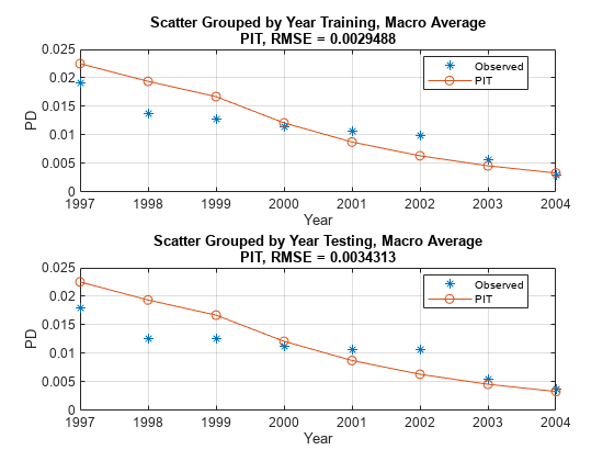
Reset original values of the GDP and Market variables. The TTC PD values predicted using the PIT model and median or mean macro values are stored in the TTCPD2 column and that column is used to compare the predictions against other models below.
data.GDP = [];
data.Market = [];
data = join(data,dataMacro);
disp(head(data,10))
    ID    ScoreGroup     YOB    Default    Year      TTCPD        PITPD       TTCPD2       GDP     Market
    __    ___________    ___    _______    ____    _________    _________    _________    _____    ______

    1     Low Risk        1        0       1997    0.0084797    0.0093187     0.010688     2.72      7.61
    1     Low Risk        2        0       1998    0.0067697     0.005349    0.0077772     3.57     26.24
    1     Low Risk        3        0       1999    0.0054027    0.0044938    0.0056548     2.86      18.1
    1     Low Risk        4        0       2000    0.0043105    0.0038285    0.0041093     2.43      3.19
    1     Low Risk        5        0       2001    0.0034384    0.0035402    0.0029848     1.26    -10.51
    1     Low Risk        6        0       2002    0.0027422    0.0035259    0.0021674    -0.59    -22.95
    1     Low Risk        7        0       2003    0.0021867    0.0018336    0.0015735     0.63      2.78
    1     Low Risk        8        0       2004    0.0017435    0.0010921    0.0011422     1.85      9.48
    2     Medium Risk     1        0       1997     0.015097     0.016554     0.018966     2.72      7.61
    2     Medium Risk     2        0       1998     0.012069    0.0095319     0.013833     3.57     26.24
Compare the Models
First, compare the two versions of the TTC model.
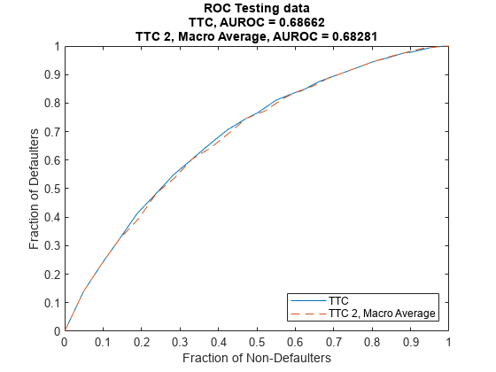
Compare the model discrimination using modelDiscriminationPlot. The two models have very similar performance ranking customers, as measured by the receiver operating characteristic (ROC) curve and the area under the ROC curve (AUROC, or simply AUC) metric.
figure;
modelDiscriminationPlot(TTCModel,data(TestDataInd,:),"DataID",'Testing data',"ReferencePD",data.TTCPD2(TestDataInd),"ReferenceID",'TTC 2, Macro Average')
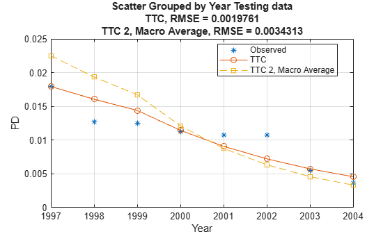
However, the TTC model is more accurate, the predicted PD values are closer to the observed default rates. The plot generated using modelCalibrationPlot demonstrates that the root mean squared error (RMSE) reported in the plot confirms the TTC model is more accurate for this data set.
modelCalibrationPlot(TTCModel,data(TestDataInd,:),'Year',"DataID",'Testing data',"ReferencePD",data.TTCPD2(TestDataInd),"ReferenceID",'TTC 2, Macro Average')
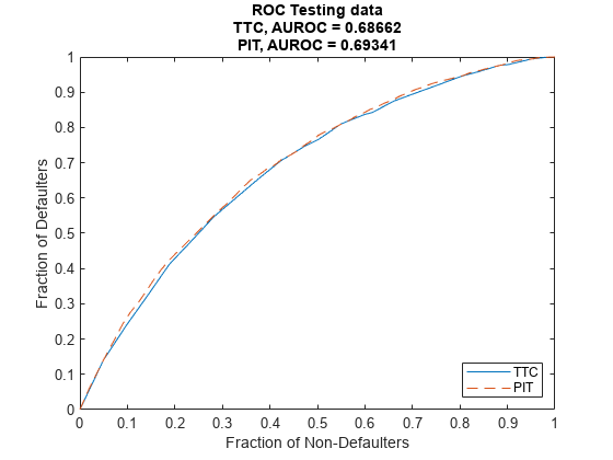
Use modelDiscriminationPlot to compare the TTC model and the PIT model.
The AUROC is only slightly better for the PIT model, showing that both models are comparable regarding ranking customers by risk.
figure;
modelDiscriminationPlot(TTCModel,data(TestDataInd,:),"DataID",'Testing data',"ReferencePD",data.PITPD(TestDataInd),"ReferenceID",'PIT')
Use modelCalibrationPlot to visualize the model accuracy, or model calibration. The plot shows that the PIT model performs much better, with predicted PD values much closer to the observed default rates. This is expected, since the predictions are sensitive to the macro variables, whereas the TTC model only uses the initial score and the age of the model to make predictions.
modelCalibrationPlot(TTCModel,data(TestDataInd,:),'Year',"DataID",'Testing data',"ReferencePD",data.PITPD(TestDataInd),"ReferenceID",'PIT')

You can use modelDiscrimination to programmatically access the AUROC and the RMSE without creating a plot.
DiscMeasure = modelDiscrimination(TTCModel,data(TestDataInd,:),"DataID",'Testing data',"ReferencePD",data.PITPD(TestDataInd),"ReferenceID",'PIT');
disp(DiscMeasure)
                          AUROC
                         _______

    TTC, Testing data    0.68662
    PIT, Testing data    0.69341
CalMeasure = modelCalibration(TTCModel,data(TestDataInd,:),'Year',"DataID",'Testing data',"ReferencePD",data.PITPD(TestDataInd),"ReferenceID",'PIT');
disp(CalMeasure)
                                            RMSE
                                          _________

    TTC, grouped by Year, Testing data    0.0019761
    PIT, grouped by Year, Testing data    0.0006322
Although all models have comparable discrimination power, the accuracy of the PIT model is much better. However, TTC and PIT models are often used for different purposes, and the TTC model may be preferred if having more stable predictions over time is important.
References
Generalized Linear Models documentation, see Generalized Linear Models.
Baesens, B., D. Rosch, and H. Scheule. Credit Risk Analytics. Wiley, 2016.