plot

Plot normalized bistatic reflectivity

Since R2026a

Syntax

plot(brefl)

plot(brefl,mode)

plot(___,Name=Value)

Description

plot(brefl) plots normalized bistatic radar cross section (NBRCS) values from the input bistaticSurfaceReflectivityLand object brefl as a function of geometry at a single frequency .

plot(brefl,mode) also specifies the type of model, mode, with options of "InPlane" or "OutOfPlane".

plot(___,Name=Value) specifies additional options using one or more name-value arguments.

Examples

Plot In-Plane and Out-of-Plane Land Surface Models

Create a bistatic reflectivity object using the Domville model for rural land and plot in-plane and out-of-plane normalized bistatic radar cross section (NBRCS) model values.

brefl = bistaticSurfaceReflectivityLand(InPlaneModel="Domville",...
        InPlaneLandType="Rural",OutOfPlaneModel="RuralInterpolation");

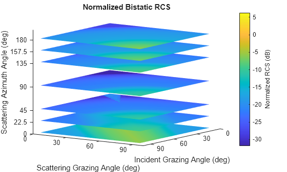
Plot the in-plane and out-of-plane models. For the out-of-plane model, display azimuths of 0, 22.5, 45, 90, 135, 157.5, and 180 degrees.

plot(brefl,"InPlane")

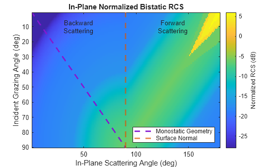
plot(brefl,Azimuth=[0 22.5 45 90 135 157.5 180])

Generate and Plot Custom In-Plane Model

Define a custom function called in_plane_bartonFarm and use a gamma value of -15 dB at 10 GHz for reference. This value is taken from the surfaceReflectivityLand "Barton" Model "Farm" LandType. The custom function converts the gamma value to linear units and adds a frequency dependence. Then it uses bsxfun to modify the gamma value based on the bistatic geometry. [1] suggests that you can use the geometric mean of the monostatic normalized radar cross section (RCS) to generate a custom in-plane normalized bistatic RCS model for backscattering bistatic geometries.

function nbrcs = in_plane_bartonFarm(angIn,angScat,freq)
    inOutAngles = [angIn, angScat];
    gammaCdB = -15; 
    gammaCdB = gammaCdB + 5*log10(freq./10e9);
    gammaC = db2pow(gammaCdB); 
    nbrcs = bsxfun(@times,gammaC,sqrt(prod(sind(inOutAngles),2))); 
end

Create a bistaticSurfaceReflectiivityLand object and set the custom in-plane function handle to @in_plane_bartonFarm.

bref = bistaticSurfaceReflectivityLand(InPlaneModel="Custom",...
       CustomInPlaneFcn=@in_plane_bartonFarm)

bref = 
  bistaticSurfaceReflectivityLand with properties:

        InPlaneModel: 'Custom'
    CustomInPlaneFcn: @in_plane_bartonFarm
     OutOfPlaneModel: 'RuralInterpolation'
             Speckle: 'None'

Plot in-plane NBRCS values at 20 GHz.

bref.plot("InPlane",Frequency=20e9)

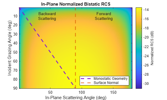
Return NBRCS values at specified bistatic configurations and frequencies.

nbrcs=bref([45;40],45,180,[20e9 21e9])

nbrcs = 2×2

    0.0319    0.0327
    0.0304    0.0311

[1] Barton, David K. "Land Clutter Models for Radar Design and Analysis." Proceedings of the IEEE 73, no. 2 (1985): 198-204.

Input Arguments

brefl — Normalized bistatic reflectivity

bistaticSurfaceReflectivity object

Normalized bistatic reflectivity, specified as a bistaticSurfaceReflectivityLand System object™.

mode — Type of model

"OutOfPlane" (default) | "InPlane"

Type of land reflectivity model to plot, specified as one of "OutOfPlane" or "InPlane". The default value is "OutOfPlane".

"OutOfPlane" refers to bistatic configurations in which the transmitter and receiver positions are non-coplanar (see Out-of-Plane Geometry for more information).

"InPlane" refers to bistatic configurations in which the transmitter and receiver lie in the same plane (see In-Plane Geometry for more information).

Plots dimensions are determined by the mode:

• "OutOfPlane" — Plots NBRCS values in dB as a function of incident grazing angle (0 – 90°) and scattering grazing angle (0 – 90°) at default scattering azimuth angles (0, 45, 90, 135, and 180°). You can specify scattering azimuth angles at which to evaluate brefl using the Azimuth name-value argument.

• "InPlane" — Plots NBRCS values in dB as a function of incident grazing angle (0 – 90°) and in-plane scattering angle (0 – 180°). The in-plane scattering angle is defined as the angle between the projection of the incident ray onto the surface and the scattered ray. Bistatic configurations are considered to be backscattering for in-plane scattering angles of 0 to 90° and forward scattering for in-plane scattering angles of 90 to 180° (see θ description in In-Plane Geometry for more information).

Data Types: char | string

Name-Value Arguments

Specify optional pairs of arguments as Name1=Value1,...,NameN=ValueN, where Name is the argument name and Value is the corresponding value. Name-value arguments must appear after other arguments, but the order of the pairs does not matter.

Example: plot(brefl,"OutOfPlane",Azimuth=[0 45 90 135 180])

Frequency — Frequency (Hz)

9.4e9 (default) | positive scalar

Frequency at which to evaluate brefl, specified as a positive scalar. When the InPlaneLandModel property is set to "Domville", valid frequencies are in the X-band, and changing the frequency does not impact returned NBRCS values. In other words, specifying a frequency is only relevant if the brefl InPlaneModel or OutofPlaneModel property is set to "Custom". The default value is 9.4 GHz.

Data Types: double

Azimuth — Scattering azimuth angles for "OutOfPlane" mode (degrees)

[0:45:180] (default) | scalar in the range of [-180,180] | row vector

Scattering azimuth angles at which to evaluate and plot brefl for the "OutOfPlane" mode, specified as a scalar or row vector, with values between –180° and 180°. The scattering azimuth angle is the angle between the projection of the incident ray onto the surface and the projection of the scattered ray onto the surface. See Out-of-Plane Geometry for more information. This name-value argument is only available when the input mode is set to "OutOfPlane". Default values are 0, 45, 90, 135, and 180°. Units are in degrees.

Data Types: double

Parent — Handle to axes in figure

current axes (default) | Axes object

Handle to the plot axes, specified as an Axes object. Use the gca function to get and set properties of the current axes.

More About

In-Plane Geometry

The plots below provide example in-plane bistatic configurations in which transmitted (black) and received (blue) signals lie in the same plane. The incident grazing angle AngIn and the scattering grazing angle AngScat are input arguments that are measured relative to the surface plane, with values that can vary between 0 and 90°. The in-plane scattering angle θ (Theta) is relevant to the CustomInPlaneFcn and plot method and is shown in green. θ is measured from the same surface as AngIn and is defined as the angle between the projection of the incident ray onto the surface and the scattered ray, with values that can vary between 0 and 180°. For backscattering configurations, θ is equivalent to AngScat and for forward scattering configurations, θ is equal to 180 - AngScat. The surface normal is shown for reference. Note: plots are shown with flat ground surfaces for simplicity. Tilted surfaces will modify AngIn and AngScat, similar to the effect illustrated for the monostatic Grazing Angle.

Backscattering geometries occur when the receiver is positioned to receive surface reflections that are scattered back towards the direction of the transmitter and forward scattering geometries occur when reflections that continue to travel away from the transmitter are received. Bistatic configurations are considered to be backscattering for AngAz values of 180 or –180° (left and right plots) and forward scattering when the AngAz value is 0° (middle plot). The backscattering azimuths correspond to θ values between 0 and 90° and the forward scattering azimuth of 0° corresponds to θ values between 90 and 180°.

Out-of-Plane Geometry

The 3-D plots below provide example out-of-plane bistatic configurations for transmitter positions shown in black and receiver positions in blue. The incident grazing angle AngIn and the scattering grazing angle AngScat are input arguments that are measured relative to the surface plane, with values that can vary between 0 and 90°. The scattering azimuth AngAz, shown in orange, is the angle between the projection of the incident ray onto the surface and the projection of the scattered ray onto the surface. Following the right-hand rule convention, positive AngAz angles are measured counterclockwise from the projection of the incident ray onto the surface. The surface normal is shown for reference. Note: plots are shown with flat ground surfaces for simplicity. Tilted surfaces will modify AngIn and AngScat, similar to the effect illustrated for the monostatic Grazing Angle.

Backscattering geometries occur when the receiver is positioned to receive surface reflections that are scattered back towards the direction of the transmitter and forward scattering geometries occur when reflections that continue to travel away from the transmitter are received. Bistatic configurations are considered to be backscattering for AngAz values of 90 to 180° and –90 to –180° and forward scattering for AngAz values of 0 to 90° and 0 to –90°.

Version History

Introduced in R2026a