Simulink を使用した故障データの生成
この例では、Simulink® モデルを使用して故障データと健全データを生成する方法を説明します。故障データと健全データを使用して、状態監視のアルゴリズムを開発します。例ではトランスミッション システムを使用してギア歯、センサー ドリフト、およびシャフト摩耗の故障をモデル化します。
トランスミッション システム モデル
トランスミッション ケーシング モデルでは、Simscape™ Driveline™ ブロックを使用して単純なトランスミッション システムをモデル化します。トランスミッション システムは、トルク ドライブ、ドライブ シャフト、クラッチ、および出力シャフトに接続されている高速ギアと低速ギアで構成されます。
mdl = 'pdmTransmissionCasing';
open_system(mdl)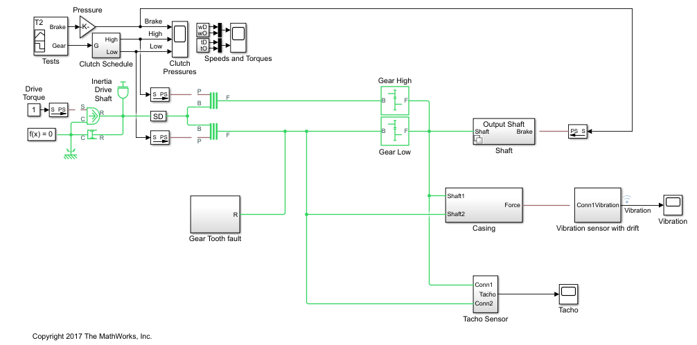
トランスミッション システムにはケーシングの振動を監視する振動センサーが含まれています。ケーシング モデルはシャフトの角変位をケーシングの線形変位に変換します。ケーシングはバネ質量ダンパー システムとしてモデル化され、ケーシングからの振動 (ケーシング加速度) が測定されます。
open_system([mdl '/Casing'])

故障のモデル化
トランスミッション システムには、振動センサー ドリフト、ギア歯の故障、およびシャフト摩擦の各故障モデルが含まれています。センサー ドリフトの故障は、センサー モデルにオフセットを導入することで簡単にモデル化されます。オフセットはモデル変数 SDrift によって制御されます。SDrift=0 はセンサー故障がないことを意味する点に注意してください。
open_system([mdl '/Vibration sensor with drift'])
シャフト摩耗の故障はバリアント サブシステムによってモデル化されます。ここではサブシステム バリアントがシャフト減衰を変更しますが、バリアント サブシステムを使用してシャフト モデルの実装を完全に変えることもできます。選択したバリアントはモデル変数 ShaftWear によって制御されます。ShaftWear=0 はシャフト故障がないことを意味する点に注意してください。
open_system([mdl '/Shaft'])
open_system([mdl,'/Shaft/Output Shaft'])
ギア歯の故障は、ドライブ シャフトの回転における固定位置に外乱トルクを挿入することでモデル化されます。シャフト位置はラジアン単位で測定され、シャフト位置が 0 近傍の小さいウィンドウ内にあるとシャフトに外乱力が適用されます。外乱の大きさはモデル変数 ToothFaultGain によって制御されます。ToothFaultGain=0 はギア歯の故障がないことを意味する点に注意してください。

故障データと健全データのシミュレーション
トランスミッション モデルは、センサー ドリフト、ギア歯、およびシャフト摩耗という 3 つの異なる故障タイプの存在と重大度を制御する変数を使って構成されます。モデル変数 SDrift、ToothFaultGain、および ShaftWear を変化させることで、各種故障タイプの振動データを作成できます。Simulink.SimulationInput オブジェクトの配列を使用して、いくつかの異なるシミュレーション シナリオを定義します。たとえば、各モデル変数の値の配列を選択してから、関数 ndgrid を使用して、モデル変数値の各組み合わせに対し Simulink.SimulationInput を作成します。
toothFaultArray = -2:2/10:0; % Tooth fault gain values
sensorDriftArray = -1:0.5:1; % Sensor drift offset values
shaftWearArray = [0 -1];       % Variants available for drive shaft conditions

% Create an n-dimensional array with combinations of all values
[toothFaultValues,sensorDriftValues,shaftWearValues] = ...
    ndgrid(toothFaultArray,sensorDriftArray,shaftWearArray);

for ct = numel(toothFaultValues):-1:1
    % Create a Simulink.SimulationInput for each combination of values
    siminput = Simulink.SimulationInput(mdl);

    % Modify model parameters
    siminput = setVariable(siminput,'ToothFaultGain',toothFaultValues(ct));
    siminput = setVariable(siminput,'SDrift',sensorDriftValues(ct));
    siminput = setVariable(siminput,'ShaftWear',shaftWearValues(ct));

    % Collect the simulation input in an array
    gridSimulationInput(ct) = siminput;
end
同様に、各モデル変数の乱数値の組み合わせを作成します。3 つの故障タイプのうち一部のみを表す組み合わせができるように、必ず 0 値を含めるようにします。
rng('default'); % Reset random seed for reproducibility
toothFaultArray = [0 -rand(1,6)];    % Tooth fault gain values
sensorDriftArray = [0 randn(1,6)/8]; % Sensor drift offset values
shaftWearArray = [0 -1];               % Variants available for drive shaft conditions

%Create an n-dimensional array with combinations of all values
[toothFaultValues,sensorDriftValues,shaftWearValues] = ...
    ndgrid(toothFaultArray,sensorDriftArray,shaftWearArray);

for ct=numel(toothFaultValues):-1:1
    % Create a Simulink.SimulationInput for each combination of values
    siminput = Simulink.SimulationInput(mdl);

    % Modify model parameters
    siminput = setVariable(siminput,'ToothFaultGain',toothFaultValues(ct));
    siminput = setVariable(siminput,'SDrift',sensorDriftValues(ct));
    siminput = setVariable(siminput,'ShaftWear',shaftWearValues(ct));

    % Collect the simulation input in an array
    randomSimulationInput(ct) = siminput;
end
Simulink.SimulationInput オブジェクトの配列を定義したら、関数 generateSimulationEnsemble を使用してシミュレーションを実行します。関数 generateSimulationEnsemble は、ログ データをファイルに保存し、信号のログに timetable 形式を使用して、保存ファイルに Simulink.SimulationInput オブジェクトを格納するようモデルを構成します。関数 generateSimulationEnsemble は、シミュレーションが正常に完了したかどうかを示すステータス フラグを返します。
上記のコードは、グリッドの変数値から 110 のシミュレーション入力、ランダム変数の値から 98 のシミュレーション入力を作成し、合計 208 のシミュレーションが提供されています。これら 208 のシミュレーションを並列実行すると、標準的なデスクトップでは 2 時間以上かかる場合があり、約 10 GB のデータが生成されます。便宜上、最初の 10 個のシミュレーションのみを実行するオプションが用意されています。
% Run the simulations and create an ensemble to manage the simulation results
if ~exist(fullfile(pwd,'Data'),'dir')
    mkdir(fullfile(pwd,'Data')) % Create directory to store results
end
runAll = true;
if runAll
   [ok,e] = generateSimulationEnsemble([gridSimulationInput, randomSimulationInput], ...
        fullfile(pwd,'Data'),'UseParallel', true, 'ShowProgress', false);
else
    [ok,e] = generateSimulationEnsemble(gridSimulationInput(1:10), fullfile(pwd,'Data'), 'ShowProgress', false); %#ok<*UNRCH>
end
Starting parallel pool (parpool) using the 'Processes' profile ...
Preserving jobs with IDs: 1 because they contain crash dump files.
You can use 'delete(myCluster.Jobs)' to remove all jobs created with profile Processes. To create 'myCluster' use 'myCluster = parcluster('Processes')'.
Connected to parallel pool with 6 workers.
generateSimulationEnsemble が実行され、シミュレーションの結果をログに記録しました。simulationEnsembleDatastore コマンドを使用して、シミュレーション結果を処理して解析するためのシミュレーション アンサンブルを作成します。
ens = simulationEnsembleDatastore(fullfile(pwd,'Data'));シミュレーション結果の処理
simulationEnsembleDatastore コマンドによって、シミュレーション結果を指すアンサンブル オブジェクトが作成されました。アンサンブル オブジェクトを使用して、アンサンブルの各メンバーに含まれるデータの準備と解析を行います。アンサンブル オブジェクトはアンサンブル内のデータ変数をリストし、既定ではすべての変数が読み取り対象として選択されています。
ens
ens =
  simulationEnsembleDatastore with properties:

           DataVariables: [6×1 string]
    IndependentVariables: [0×0 string]
      ConditionVariables: [0×0 string]
       SelectedVariables: [6×1 string]
                ReadSize: 1
              NumMembers: 208
          LastMemberRead: [0×0 string]
                   Files: [208×1 string]
ens.SelectedVariables
ans = 6×1 string array
    "SimulationInput"
    "SimulationMetadata"
    "Tacho"
    "Vibration"
    "xFinal"
    "xout"
解析のため、Vibration 信号と Tacho 信号、および Simulink.SimulationInput のみを読み取ります。Simulink.SimulationInput はシミュレーションに使用されるモデル変数の値を含み、アンサンブル メンバーの故障ラベルを作成するために使われます。アンサンブルの read コマンドを使用してアンサンブル メンバーのデータを取得します。
ens.SelectedVariables = ["Vibration" "Tacho" "SimulationInput"];
data = read(ens)
data=1×3 table
    40272×1 timetable    40272×1 timetable    1×1 SimulationInput
返されたデータから振動信号を抽出し、それをプロットします。
vibration = data.Vibration{1};
plot(vibration.Time,vibration.Data)
title('Vibration')
ylabel('Acceleration')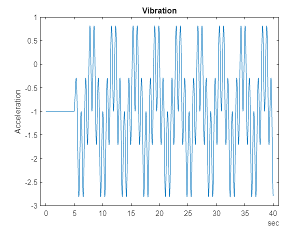
シミュレーションの最初の 10 秒にはトランスミッション システムが起動している最中のデータが含まれるため、解析ではこのデータを破棄します。
idx = vibration.Time >= seconds(10);
vibration = vibration(idx,:);
vibration.Time = vibration.Time - vibration.Time(1);
Tacho 信号には、ドライブおよび負荷シャフトの回転のパルスが含まれますが、解析 (具体的には、時間同期平均化) にはシャフト回転の時間が必要です。次のコードは、Tacho データの最初の 10 秒を破棄して tachoPulses 内のシャフト回転時間を検出します。
tacho = data.Tacho{1};
idx = tacho.Time >= seconds(10);
tacho = tacho(idx,:);
plot(tacho.Time,tacho.Data)
title('Tacho pulses')
legend('Drive shaft','Load shaft') % Load shaft rotates more slowly than drive shaft
idx = diff(tacho.Data(:,2)) > 0.5;
tachoPulses = tacho.Time(find(idx)+1)-tacho.Time(1)
tachoPulses = 8×1 duration array
    "2.8543 sec"
    "6.6508 sec"
    "10.447 sec"
    "14.244 sec"
    "18.04 sec"
    "21.837 sec"
    "25.634 sec"
    "29.43 sec"
Simulink.SimulationInput.Variables プロパティはシミュレーションに使用された故障パラメーターの値を含み、これらの値によって各アンサンブル メンバーに故障ラベルを作成できるようになります。
vars = data.SimulationInput{1}.Variables;
idx = strcmp({vars.Name},'SDrift');
if any(idx)
    sF = abs(vars(idx).Value) > 0.01; % Small drift values are not faults
else
    sF = false;
end
idx = strcmp({vars.Name},'ShaftWear');
if any(idx)
    sV = vars(idx).Value < 0;
else
    sV = false;
end
if any(idx)
    idx = strcmp({vars.Name},'ToothFaultGain');
    sT = abs(vars(idx).Value) > 0.1; % Small tooth fault values are not faults
else
    sT = false
end
faultCode = sF + 2*sV + 4*sT; % A fault code to capture different fault conditions
処理された振動信号とタコ信号および故障ラベルが、後で使用するためアンサンブルに追加されます。
sdata = table({vibration},{tachoPulses},sF,sV,sT,faultCode, ...
'VariableNames',{'Vibration','TachoPulses','SensorDrift','ShaftWear','ToothFault','FaultCode'}) sdata=1×6 table
30106×1 timetable 8×1 duration 1 0 0 1
ens.DataVariables = [ens.DataVariables; "TachoPulses"];アンサンブルの ConditionVariables プロパティを使用して、状態または故障ラベル データを含んでいるアンサンブル内の変数を識別できます。新たに作成された故障ラベルを含むようにプロパティを設定します。
ens.ConditionVariables = ["SensorDrift","ShaftWear","ToothFault","FaultCode"];
上記のコードはアンサンブルの 1 つのメンバーを処理するために使用しました。アンサンブルのすべてのメンバーを処理するには、上のコードを関数 prepareData に変換し、アンサンブルの hasdata コマンドとループを使用して prepareData をすべてのアンサンブル メンバーに適用します。アンサンブルを分割して並列処理することにより、アンサンブル メンバーを並列で処理できます。
reset(ens)
runLocal = false;
if runLocal
    % Process each member in the ensemble
    while hasdata(ens)
        data = read(ens);
        addData = prepareData(data);
        writeToLastMemberRead(ens,addData)
    end
else
    % Split the ensemble into partitions and process each partition in parallel
    n = numpartitions(ens,gcp);
    parfor ct = 1:n
        subens = partition(ens,n,ct);
        while hasdata(subens)
            data = read(subens);
            addData = prepareData(data);
            writeToLastMemberRead(subens,addData)
        end
    end
end
hasdata コマンドと read コマンドを使用して振動信号を抽出し、アンサンブルの 10 個おきのメンバーの振動信号をプロットします。
reset(ens)
ens.SelectedVariables = "Vibration";
figure,
ct = 1;
while hasdata(ens)
    data = read(ens);
    if mod(ct,10) == 0
        vibration = data.Vibration{1};
        plot(vibration.Time,vibration.Data)
        hold on
    end
    ct = ct + 1;
end
hold off
title('Vibration signals')
ylabel('Acceleration')

シミュレーション データの解析
これでデータのクリーン アップと前処理が済み、特徴を抽出してさまざまな故障タイプの分類に使用する特徴を決定する準備ができました。まず、処理済みのデータのみを返すようにアンサンブルを構成します。
ens.SelectedVariables = ["Vibration","TachoPulses"];
アンサンブルの各メンバーにつき、いくつかの時間およびスペクトル ベースの特徴を計算します。これには、信号の平均値、分散、ピーク ツー ピークなどの信号統計、近似エントロピーおよびリアプノフ指数などの非線形の信号特性、振動信号の時間同期平均のピーク周波数および時間同期平均包絡線信号の強度などのスペクトル特性が含まれます。関数 analyzeData には、抽出される特徴の完全なリストが含まれます。例として、時間同期平均化された振動信号のスペクトルを計算することを検討します。
reset(ens)
data = read(ens)
data=1×2 table
    30106×1 timetable    8×1 duration
vibration = data.Vibration{1};

% Interpolate the Vibration signal onto periodic time base suitable for fft analysis
np = 2^floor(log(height(vibration))/log(2));
dt = vibration.Time(end)/(np-1);
tv = 0:dt:vibration.Time(end);
y = retime(vibration,tv,'linear');

% Compute the time synchronous average of the vibration signal
tp = seconds(data.TachoPulses{1});
vibrationTSA = tsa(y,tp);
figure
plot(vibrationTSA.Time,vibrationTSA.tsa)
title('Vibration time synchronous average')
ylabel('Acceleration')
% Compute the spectrum of the time synchronous average
np = numel(vibrationTSA);
f = fft(vibrationTSA.tsa.*hamming(np))/np;
frTSA = f(1:floor(np/2)+1);            % TSA frequency response
wTSA = (0:np/2)/np*(2*pi/seconds(dt)); % TSA spectrum frequencies
mTSA = abs(frTSA);                     % TSA spectrum magnitudes
figure
semilogx(wTSA,20*log10(mTSA))
title('Vibration spectrum')
xlabel('rad/s')

ピーク振幅に対応する周波数は、さまざまな故障タイプの分類に役立つ特徴となる可能性があります。以下のコードでは、すべてのアンサンブル メンバーについて上記の特徴を計算します (この解析の実行には、標準的なデスクトップで最大 1 時間を要する場合があります。アンサンブルの partition コマンドを使用して並列で解析を実行する、オプションのコードが提示されています)。特徴の名前がアンサンブルのデータ変数プロパティに追加された後、writeToLastMemberRead が呼び出されて各アンサンブル メンバーに計算された特徴が追加されます。
reset(ens)
ens.DataVariables = [ens.DataVariables; ...
    "SigMean";"SigMedian";"SigRMS";"SigVar";"SigPeak";"SigPeak2Peak";"SigSkewness"; ...
    "SigKurtosis";"SigCrestFactor";"SigMAD";"SigRangeCumSum";"SigCorrDimension";"SigApproxEntropy"; ...
    "SigLyapExponent";"PeakFreq";"HighFreqPower";"EnvPower";"PeakSpecKurtosis"];
if runLocal
    while hasdata(ens)
        data = read(ens);
        addData = analyzeData(data);
        writeToLastMemberRead(ens,addData);
    end
else
    % Split the ensemble into partitions and analyze each partition in parallel
    n = numpartitions(ens,gcp);
    parfor ct = 1:n
        subens = partition(ens,n,ct);
        while hasdata(subens)
            data = read(subens);
            addData = analyzeData(data);
            writeToLastMemberRead(subens,addData)
        end
    end
end
故障分類のための特徴の選択
上で計算した特徴を使用して、各種の故障状態を分類する分類器を作成します。まず、導出された特徴と故障ラベルのみを読み取るようにアンサンブルを構成します。
featureVariables = analyzeData('GetFeatureNames');
ens.DataVariables = [ens.DataVariables; featureVariables];
ens.SelectedVariables = [featureVariables; ens.ConditionVariables];
reset(ens)
すべてのアンサンブル メンバーの特徴データを 1 つの table に集めます。
featureData = gather(tall(ens))
Evaluating tall expression using the Parallel Pool 'Processes':
- Pass 1 of 1: Completed in 14 sec
Evaluation completed in 14 sec
featureData=208×22 table
    -0.9488    -0.9722    1.3726    0.9839    0.8157    3.6314    -0.0415    2.2666    2.0514    0.8081    2.8562e+04    1.1427    0.0316     79.5312    0    6.7528e-06    3.2349e-07    162.1284    1    0    0    1
    -0.9754    -0.9896    1.3937    0.9911    0.8157    3.6314    -0.0238    2.2598    2.0203    0.8102    2.9418e+04    1.1362    0.0378     70.3389    0    5.0788e-08    9.1568e-08    226.1212    1    0    0    1
     1.0502     1.0267    1.4449    0.9849    2.8157    3.6314    -0.0416    2.2658    1.9487    0.8085    3.1710e+04    1.1479    0.0316    125.1842    0    6.7416e-06    3.1343e-07    162.1259    1    1    0    3
     1.0227     1.0045    1.4288    0.9955    2.8157    3.6314    -0.0164    2.2483    1.9707    0.8132    3.0984e+04    1.1472    0.0321    112.5155    0    4.9939e-06    2.6719e-07    162.1277    1    1    0    3
     1.0123     1.0024    1.4202    0.9923    2.8157    3.6314    -0.0147    2.2542    1.9826    0.8116    3.0661e+04    1.1470    0.0329    109.0188    0    3.6182e-06    2.1964e-07    230.3912    1    1    0    3
     1.0275     1.0102    1.4338    1.0001    2.8157    3.6314    -0.0266    2.2439    1.9638    0.8159    3.1102e+04    1.0975    0.0334     64.4981    0    2.5493e-06    1.9224e-07    230.3907    1    1    0    3
     1.0464     1.0275    1.4477    1.0011    2.8157    3.6314    -0.0428    2.2455    1.9449    0.8159    3.1665e+04    1.1417    0.0342     98.7589    0    1.7313e-06    1.6263e-07    230.3870    1    1    0    3
     1.0459     1.0257    1.4402    0.9805    2.8157    3.6314    -0.0354    2.2757    1.9550    0.8058    3.1554e+04    1.1345    0.0353     44.3035    0    1.1115e-06    1.2807e-07    230.3927    1    1    0    3
     1.0263     1.0068    1.4271    0.9834    2.8157    3.6314    -0.0165    2.2726    1.9730    0.8062    3.0951e+04    1.1515    0.0359    125.2802    0    6.5947e-07    1.2080e-07    162.1264    1    1    0    3
     1.0103     1.0014    1.4183    0.9909    2.8157    3.6314    -0.0117    2.2614    1.9853    0.8099    3.0465e+04    1.0619    0.0365     17.0927    0    5.2297e-07    1.0704e-07    230.3865    1    1    0    3
     1.0129     1.0023    1.4190    0.9876    2.8157    3.6314    -0.0110    2.2660    1.9843    0.8087    3.0523e+04    1.1371    0.0372     84.5701    0    2.1605e-07    8.5562e-08    230.3923    1    1    0    3
     1.0251     1.0104    1.4291    0.9917    2.8157    3.6314    -0.0236    2.2588    1.9702    0.8105    3.0896e+04    1.1261    0.0378     98.4616    0    5.0275e-08    9.0495e-08    230.3920    1    1    0    3
    -0.9730    -0.9924    1.3928    0.9933    0.8157    3.6314    -0.0126    2.2589    2.0216    0.8110    2.9351e+04    1.1277    0.0385     42.8867    0    1.1383e-11    8.3005e-08    230.3910    1    0    1    5
     1.0277     1.0084    1.4315    0.9931    2.8157    3.6314    -0.0135    2.2598    1.9669    0.8108    3.0963e+04    1.1486    0.0385     99.4258    0    1.1346e-11    8.3530e-08    226.1215    1    1    1    7
      ⋮
センサー ドリフト故障について考えます。上で計算したすべての特徴を予測子とし、センサー ドリフト故障のラベル (true または false の値) を応答として、fscnca コマンドを使用します。fscnca コマンドは各特徴の重みを返しますが、重みの大きい特徴は、応答を予測する上での重要度が高くなります。センサー ドリフト故障の場合、重みは、2 つの特徴が重要な予測子となり (信号の累積和範囲とスペクトル尖度のピーク周波数)、残りの特徴はほとんど影響しないことを示しています。
idxResponse = strcmp(featureData.Properties.VariableNames,'SensorDrift');
idxLastFeature = find(idxResponse)-1; % Index of last feature to use as a potential predictor
featureAnalysis = fscnca(featureData{:,1:idxLastFeature},featureData.SensorDrift);
featureAnalysis.FeatureWeights
ans = 18×1

    0.0000
    0.0000
    0.0000
    0.0000
    0.0000
    0.0000
    0.0000
    0.0000
    0.0000
    0.0000
      ⋮
idxSelectedFeature = featureAnalysis.FeatureWeights > 0.1;
classifySD = [featureData(:,idxSelectedFeature), featureData(:,idxResponse)]
classifySD=208×3 table
    2.8562e+04    162.1284    1
    2.9418e+04    226.1212    1
    3.1710e+04    162.1259    1
    3.0984e+04    162.1277    1
    3.0661e+04    230.3912    1
    3.1102e+04    230.3907    1
    3.1665e+04    230.3870    1
    3.1554e+04    230.3927    1
    3.0951e+04    162.1264    1
    3.0465e+04    230.3865    1
    3.0523e+04    230.3923    1
    3.0896e+04    230.3920    1
    2.9351e+04    230.3910    1
    3.0963e+04    226.1215    1
      ⋮
累積和範囲のグループ化されたヒストグラムから、この特徴がなぜセンサー ドリフト故障の重要な予測子であるかを把握することができます。
figure
histogram(classifySD.SigRangeCumSum(classifySD.SensorDrift),'BinWidth',5e3)
xlabel('Signal cumulative sum range')
ylabel('Count')
hold on
histogram(classifySD.SigRangeCumSum(~classifySD.SensorDrift),'BinWidth',5e3)
hold off
legend('Sensor drift fault','No sensor drift fault')

ヒストグラム プロットには、信号の累積和範囲がセンサー ドリフト故障の検出に適した特徴でありながら、センサー ドリフトの分類に信号の累積和範囲だけを使用すると信号の累積和範囲が 0.5 より小さい場合に誤検知の可能性があるため、おそらく追加の特徴が必要となることが示されています。
シャフト摩耗故障について考えます。ここでは関数 fscnca が、故障の重要な予測子となる 3 つの特徴 (信号のリアプノフ指数、ピーク周波数、スペクトル尖度のピーク周波数) があることを示しており、シャフト摩耗故障を分類するにはこれらを選択します。
idxResponse = strcmp(featureData.Properties.VariableNames,'ShaftWear');
featureAnalysis = fscnca(featureData{:,1:idxLastFeature},featureData.ShaftWear);
featureAnalysis.FeatureWeights
ans = 18×1
0.0000
0.0000
0.0000
0.0000
0.0000
0.0000
0.0000
0.0000
0.0000
0.0000
⋮
idxSelectedFeature = featureAnalysis.FeatureWeights > 0.1;
classifySW = [featureData(:,idxSelectedFeature), featureData(:,idxResponse)]
classifySW=208×4 table
     79.5312    0    162.1284    0
     70.3389    0    226.1212    0
    125.1842    0    162.1259    1
    112.5155    0    162.1277    1
    109.0188    0    230.3912    1
     64.4981    0    230.3907    1
     98.7589    0    230.3870    1
     44.3035    0    230.3927    1
    125.2802    0    162.1264    1
     17.0927    0    230.3865    1
     84.5701    0    230.3923    1
     98.4616    0    230.3920    1
     42.8867    0    230.3910    0
     99.4258    0    226.1215    1
      ⋮
信号のリアプノフ指数のグループ化されたヒストグラムには、この特徴だけでは適切な予測子とならない理由が示されます。
figure
histogram(classifySW.SigLyapExponent(classifySW.ShaftWear))
xlabel('Signal lyapunov exponent')
ylabel('Count')
hold on
histogram(classifySW.SigLyapExponent(~classifySW.ShaftWear))
hold off
legend('Shaft wear fault','No shaft wear fault')

シャフト摩耗の特徴選択は、シャフト摩耗の故障を分類するには複数の特徴が必要であることを示します。これはグループ化されたヒストグラムから確認でき、最も重要な特徴 (ここではリアプノフ指数) の分布が故障シナリオと故障なしのシナリオの両方で類似しているため、この故障を正しく分類するには追加の特徴が必要であることがわかります。
最後に、ギア歯の故障について考慮します。関数 fscnca は、故障の重要な予測子となる特徴が主に 3 つあること (信号の累積和範囲、信号のリアプノフ指数、スペクトル尖度のピーク周波数) を示しています。ギア歯の故障を分類するためにこれら 3 つの特徴を選択すると、結果として性能の悪い分類器となります。代わりに、最も重要な特徴を 6 つ使用します。
idxResponse = strcmp(featureData.Properties.VariableNames,'ToothFault');
featureAnalysis = fscnca(featureData{:,1:idxLastFeature},featureData.ToothFault);
[~,idxSelectedFeature] = sort(featureAnalysis.FeatureWeights);
classifyTF = [featureData(:,idxSelectedFeature(end-5:end)), featureData(:,idxResponse)]classifyTF=208×7 table
0.8157 0 1.1427 79.5312 162.1284 2.8562e+04 0
0.8157 0 1.1362 70.3389 226.1212 2.9418e+04 0
2.8157 0 1.1479 125.1842 162.1259 3.1710e+04 0
2.8157 0 1.1472 112.5155 162.1277 3.0984e+04 0
2.8157 0 1.1470 109.0188 230.3912 3.0661e+04 0
2.8157 0 1.0975 64.4981 230.3907 3.1102e+04 0
2.8157 0 1.1417 98.7589 230.3870 3.1665e+04 0
2.8157 0 1.1345 44.3035 230.3927 3.1554e+04 0
2.8157 0 1.1515 125.2802 162.1264 3.0951e+04 0
2.8157 0 1.0619 17.0927 230.3865 3.0465e+04 0
2.8157 0 1.1371 84.5701 230.3923 3.0523e+04 0
2.8157 0 1.1261 98.4616 230.3920 3.0896e+04 0
0.8157 0 1.1277 42.8867 230.3910 2.9351e+04 1
2.8157 0 1.1486 99.4258 226.1215 3.0963e+04 1
⋮
figure
histogram(classifyTF.SigRangeCumSum(classifyTF.ToothFault))
xlabel('Signal cumulative sum range')
ylabel('Count')
hold on
histogram(classifyTF.SigRangeCumSum(~classifyTF.ToothFault))
hold off
legend('Gear tooth fault','No gear tooth fault')

上記を使用すると、結果としてギア歯の故障を分類する多項式 svm が得られます。特徴テーブルを、学習に使用されるメンバーとテストおよび検証に使用されるメンバーに分割します。学習用メンバーを使用して、fitcsvm コマンドで svm 分類器を作成します。
rng('default') % For reproducibility
cvp = cvpartition(size(classifyTF,1),'KFold',5); % Randomly partition the data for training and validation
classifierTF = fitcsvm(...
    classifyTF(cvp.training(1),1:end-1), ...
    classifyTF(cvp.training(1),end), ...
    'KernelFunction','polynomial', ...
    'PolynomialOrder',2, ...
    'KernelScale','auto', ...
    'BoxConstraint',1, ...
    'Standardize',true, ...
    'ClassNames',[false; true]);
この分類器を使用して、predict コマンドでテスト ポイントを分類し、混同行列を使って予測の性能をチェックします。
% Use the classifier on the test validation data to evaluate performance
actualValue = classifyTF{cvp.test(1),end};
predictedValue = predict(classifierTF, classifyTF(cvp.test(1),1:end-1));

% Check performance by computing and plotting the confusion matrix
confdata = confusionmat(actualValue,predictedValue);
h = heatmap(confdata, ...
    'YLabel', 'Actual gear tooth fault', ...
    'YDisplayLabels', {'False','True'}, ...
    'XLabel', 'Predicted gear tooth fault', ...
    'XDisplayLabels', {'False','True'}, ...
    'ColorbarVisible','off');

混同行列は、分類器によって故障なしの状態はすべて正しく分類されるものの、故障と予期される状態の 1 つが故障なしとして誤分類されることを示しています。分類器で使用される特徴の数を増やすことにより、性能をさらに改善することができます。
まとめ
この例では、シミュレーション アンサンブルを使ってシミュレーション データのクリーン アップと特徴の抽出を行い、Simulink から故障データを生成するためのワークフローを説明しました。その後、抽出した特徴を使用して、異なった故障タイプ用の分類器を作成しました。