Receiver Operating Characteristics
Receiver Operating Characteristic (ROC) curves present graphical summaries of a detector's performance. You can generate ROC curves using the rocpfa and rocsnr functions.
If you are interested in examining the effect of varying the false-alarm probability on the probability of detection for a fixed SNR, you can use rocsnr. For example, the threshold SNR for the Neyman-Pearson detector of a single sample in real-valued Gaussian noise is approximately 13.5 dB. Use rocsnr to plot the probability of detection varies as a function of the false-alarm rate at that SNR.
T = npwgnthresh(1e-6,1,'real');
rocsnr(T,'SignalType','real')

The ROC curve lets you easily read off the probability of detection for a given false-alarm rate.
You can use rocsnr to examine detector performance for different received signal types at a fixed SNR.
SNR = 13.54;
[Pd_real,Pfa_real] = rocsnr(SNR,'SignalType','real',...
    'MinPfa',1e-8);
[Pd_coh,Pfa_coh] = rocsnr(SNR,...
    'SignalType','NonfluctuatingCoherent',...
    'MinPfa',1e-8);
[Pd_noncoh,Pfa_noncoh] = rocsnr(SNR,'SignalType',...
    'NonfluctuatingNoncoherent','MinPfa',1e-8);
semilogx(Pfa_real,Pd_real)
hold on
grid on
semilogx(Pfa_coh,Pd_coh,'r')
semilogx(Pfa_noncoh,Pd_noncoh,'k')
xlabel('False-Alarm Probability')
ylabel('Probability of Detection')
legend('Real','Coherent','Noncoherent','location','southeast')
title('ROC Curve Comparison for Nonfluctuating RCS Target')
hold off

The ROC curves clearly demonstrate the superior probability of detection performance for coherent and noncoherent detectors over the real-valued case.
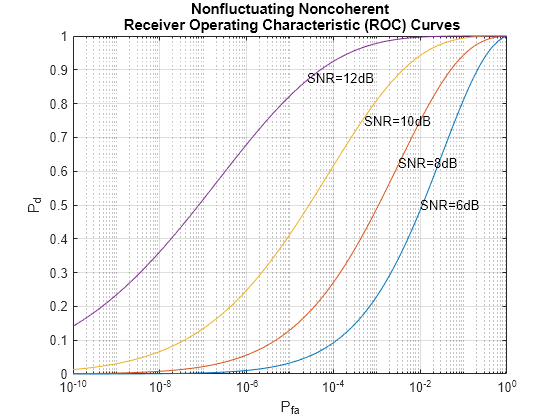
The rocsnr function accepts an SNR vector input letting you quickly examine a number of ROC curves.
SNRs = (6:2:12);
rocsnr(SNRs,'SignalType','NonfluctuatingNoncoherent')

The graph shows that, as the SNR increases, the supports of the probability distributions under the null and alternative hypotheses become more disjointed. Therefore, for a given false-alarm probability, the probability of detection increases.
You can examine the probability of detection as a function of SNR for a fixed false-alarm probability with rocpfa. To obtain ROC curves for a Swerling I target model at false-alarm probabilities of (1e-6,1e-4,1e-2,1e-1), use
Pfa = [1e-6 1e-4 1e-2 1e-1];
rocpfa(Pfa,'SignalType','Swerling1')

Use rocpfa to examine the effect of SNR on the probability of detection for a detector using noncoherent integration with a false-alarm probability of 1e-4. Assume the target has a nonfluctuating RCS and that you are integrating over 5 pulses.
[Pd,SNR] = rocpfa(1e-4,...
    'SignalType','NonfluctuatingNoncoherent',...
    'NumPulses',5);
figure;
plot(SNR,Pd); xlabel('SNR (dB)');
ylabel('Probability of Detection'); grid on;
title('Nonfluctuating Noncoherent Detector (5 Pulses)');
