Receiver Operating Characteristic (ROC) Curves Part II: Monte Carlo Simulation

This example shows how to generate a receiver operating characteristic (ROC) curve of a radar system using a Monte Carlo simulation. The ROC determines how well the system can detect targets while rejecting large spurious signal values when a target is absent (false alarms). A detection system will declare presence or absence of a target by comparing the received signal value to a preset threshold. The probability of detection (Pd) of a target is the probability that the instantaneous signal value is larger than the threshold whenever a target is actually present. The probability of false alarm (Pfa) is the probability that the signal value is larger than the threshold when a target is absent. In this case, the signal is due to noise and its properties depend on the noise statistics. The Monte Carlo simulation generates a very large number of radar returns with and without a target's presence. The simulation computes Pd and Pfa are by counting the proportion of signal values in each case that exceed the threshold.

A ROC curve plots Pd as a function of Pfa. The shape of a ROC curve depends on the received SNR of the signal. If the arriving signal SNR is known, then the ROC curve shows how well the system performs in terms of Pd and Pfa. If you specify Pd and Pfa, then you can determine how much power is needed to achieve this requirement.

You can use the function rocsnr to compute theoretical ROC curves. This example shows a ROC curve generated by a Monte Carlo simulation of a single-antenna radar system and compares that curve with a theoretical curve.

Specify Radar Requirements

Set the desired probability of detection to be 0.9 and the probability of false alarm to be $$10^{-6}$$. Set the maximum range of the radar to 4000 meters and the range resolution to 50 meters. Set the actual target range to 3000 meters. Set the target radar cross-section to 1.5 square meters and set the operating frequency to 10 GHz. All computations are performed in baseband.

c = physconst('LightSpeed');
pd = 0.9;
pfa = 1e-6;
max_range = 4000;
target_range = 3000.0;
range_res = 50;
tgt_rcs = 1.5;
fc = 10e9;
lambda = c/fc;

Any simulation that computes Pfa and pd requires processing of many signals. To keep memory requirements low, process the signals in chunks of pulses. Set the number of pulses to process to 45000 and set the size of each chunk to 10000.

Npulse = 45000;
Npulsebuffsize = 10000;

Select Waveform and Signal Parameters

Calculate the waveform pulse bandwidth using the pulse range resolution. Calculate the pulse repetition frequency from the maximum range. Because the signal is baseband, set the sampling frequency to twice the bandwidth. Calculate the pulse duration from the pulse bandwidth.

pulse_bw = c/(2*range_res);
prf = c/(2*max_range);
fs = 2*pulse_bw;
pulse_duration = 10/pulse_bw;
waveform = phased.LinearFMWaveform('PulseWidth',pulse_duration,...
    'SampleRate',fs,'SweepBandwidth',...
    pulse_bw,'PRF',prf);

Achieving a particular Pd and Pfa requires that sufficient signal power arrive at the receiver after the target reflects the signal. Compute the minimum SNR needed to achieve the specified probability of false alarm and probability of detection by using the Albersheim equation.

snr_min = albersheim(pd,pfa);

To achieve this SNR, sufficient power must be transmitted to the target. Use the radar equation to estimate the peak transmit power, peak_power, required to achieve the specified SNR in dB for the target at a range of 3000 meters. The received signal also depends on the target radar cross-section (RCS). which is assumed to follow a nonfluctuating model (Swerling 0). Set the radar to have identical transmit and receive gains of 20 dB. The radar equation is given

txrx_gain = 20;
peak_power = ((4*pi)^3*noisepow(1/pulse_duration)*target_range^4*...
    db2pow(snr_min))/(db2pow(2*txrx_gain)*tgt_rcs*lambda^2)

peak_power = 
293.1827

Set Up the Transmitter System Objects

Create System objects that make up the transmission part of the simulation: radar platform, antenna, transmitter, and radiator.

antennaplatform = phased.Platform(...
    'InitialPosition',[0; 0; 0],...
    'Velocity',[0; 0; 0]);
antenna = phased.IsotropicAntennaElement(...
    'FrequencyRange',[5e9 15e9]);
transmitter = phased.Transmitter(...
    'Gain',txrx_gain,...
    'PeakPower',peak_power,...
    'InUseOutputPort',true);
radiator = phased.Radiator(...
    'Sensor',antenna,...
    'OperatingFrequency',fc);

Set Up the Target System Object

Create a target System object™ corresponding to an actual reflecting target with a non-zero target cross-section. Reflections from this target will simulate actual radar returns. In order to compute false alarms, create a second target System object with zero radar cross section. Reflections from this target are zero except for noise.

target{1} = phased.RadarTarget(...
    'MeanRCS',tgt_rcs,...
    'OperatingFrequency',fc);
targetplatform{1} = phased.Platform(...
    'InitialPosition',[target_range; 0; 0]);
target{2} = phased.RadarTarget(...
    'MeanRCS',0,...
    'OperatingFrequency',fc);
targetplatform{2} = phased.Platform(...
    'InitialPosition',[target_range; 0; 0]);

Set Up Free-Space Propagation System Objects

Model the propagation environment from the radar to the targets and back.

channel{1} = phased.FreeSpace(...
    'SampleRate',fs,...
    'TwoWayPropagation',true,...
    'OperatingFrequency',fc);
channel{2} = phased.FreeSpace(...
    'SampleRate',fs,...
    'TwoWayPropagation',true,...
    'OperatingFrequency',fc);

Set Up Receiver System Objects

Specify the noise by setting the NoiseMethod property to 'Noise temperature' and the ReferenceTemperature property to 290 K.

collector = phased.Collector(...
    'Sensor',antenna,...
    'OperatingFrequency',fc);
receiver = phased.ReceiverPreamp(...
    'Gain',txrx_gain,...
    'NoiseMethod','Noise temperature',...
    'ReferenceTemperature',290.0,...
    'NoiseFigure',0,...
    'SampleRate',fs,...
    'EnableInputPort',true);
receiver.SeedSource = 'Property';
receiver.Seed = 2010;

Specify Fast-Time Grid

The fast-time grid is the set of time samples within one pulse repetition time interval. Each sample corresponds to a range bin.

fast_time_grid = unigrid(0,1/fs,1/prf,'[)');
rangebins = c*fast_time_grid/2;

Create Transmitted Pulse from Waveform

Create the waveform you want to transmit.

wavfrm = waveform();

Create the transmitted signal that includes transmitted antenna gains.

[sigtrans,tx_status] = transmitter(wavfrm);

Create matched filter coefficients from the waveform System object. Then create the matched filter System object.

MFCoeff = getMatchedFilter(waveform);
matchingdelay = size(MFCoeff,1) - 1;
mfilter = phased.MatchedFilter(...
    'Coefficients',MFCoeff,...
    'GainOutputPort',false);

Compute Target Range Bin

Compute the target range, and then compute the index into the range bin array. Because the target and radar are stationary, use the same values of position and velocity throughout the simulation loop. You can assume that the range bin index is constant for the entire simulation.

ant_pos = antennaplatform.InitialPosition;
ant_vel = antennaplatform.Velocity;
tgt_pos = targetplatform{1}.InitialPosition;
tgt_vel = targetplatform{1}.Velocity;
[tgt_rng,tgt_ang] = rangeangle(tgt_pos,ant_pos);
rangeidx = val2ind(tgt_rng,rangebins(2)-rangebins(1),rangebins(1));

Loop Over Pulses

Create a signal processing loop. Each step is accomplished by executing the System objects. The loop processes the pulses twice, once for the target-present condition and once for target-absent condition.

1. Radiate the signal into space using phased.Radiator.

2. Propagate the signal to the target and back to the antenna using phased.FreeSpace.

3. Reflect the signal from the target using phased.Target.

4. Receive the reflected signals at the antenna using phased.Collector.

5. Pass the received signal though the receive amplifier using phased.ReceiverPreamp. This step also adds the random noise to the signal.

6. Match filter the amplified signal using phased.MatchedFilter.

7. Store the matched filter output at the target range bin index for further analysis.

rcv_pulses = zeros(length(sigtrans),Npulsebuffsize);
h1 = zeros(Npulse,1);
h0 = zeros(Npulse,1);
Nbuff = floor(Npulse/Npulsebuffsize);
Nrem = Npulse - Nbuff*Npulsebuffsize;
for n = 1:2 % H1 and H0 Hypothesis
    trsig = radiator(sigtrans,tgt_ang);
    trsig = channel{n}(trsig,...
        ant_pos,tgt_pos,...
        ant_vel,tgt_vel);
    rcvsig = target{n}(trsig);
    rcvsig = collector(rcvsig,tgt_ang);
    
    for k = 1:Nbuff
        for m = 1:Npulsebuffsize
            rcv_pulses(:,m) = receiver(rcvsig,~(tx_status>0));
        end
        rcv_pulses = mfilter(rcv_pulses);
        rcv_pulses = buffer(rcv_pulses(matchingdelay+1:end),size(rcv_pulses,1));
        if n == 1
            h1((1:Npulsebuffsize) + (k-1)*Npulsebuffsize) = rcv_pulses(rangeidx,:).';
        else
            h0((1:Npulsebuffsize) + (k-1)*Npulsebuffsize) = rcv_pulses(rangeidx,:).';
        end
    end
    if (Nrem > 0)
        for m = 1:Nrem
            rcv_pulses(:,m) = receiver(rcvsig,~(tx_status>0));
        end
        rcv_pulses = mfilter(rcv_pulses);
        rcv_pulses = buffer(rcv_pulses(matchingdelay+1:end),size(rcv_pulses,1));
         if n == 1
            h1((1:Nrem) + Nbuff*Npulsebuffsize) = rcv_pulses(rangeidx,1:Nrem).';
        else
            h0((1:Nrem) + Nbuff*Npulsebuffsize) = rcv_pulses(rangeidx,1:Nrem).';
         end
    end
end

Create Histogram of Matched Filter Outputs

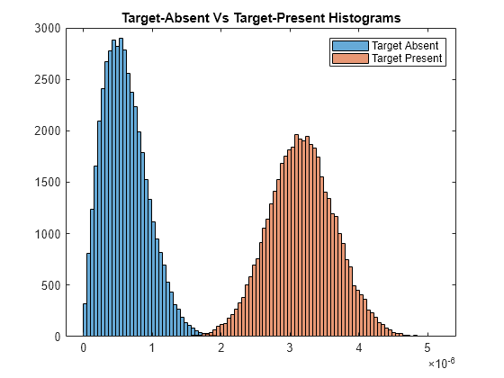
Compute histograms of the target-present and target-absent returns. Use 100 bins to give a rough estimate of the spread of signal values. Set the range of histogram values from the smallest signal to the largest signal.

h1a = abs(h1);
h0a = abs(h0);
thresh_low = min([h1a;h0a]);
thresh_hi  = max([h1a;h0a]);
nbins = 100;
binedges = linspace(thresh_low,thresh_hi,nbins);
figure
histogram(h0a,binedges)
hold on
histogram(h1a,binedges)
hold off
title('Target-Absent Vs Target-Present Histograms')
legend('Target Absent','Target Present')

Compare Simulated and Theoretical Pd and Pfa

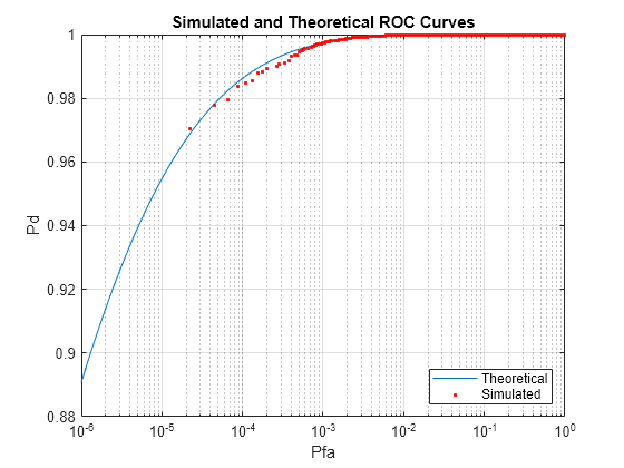
To compute Pd and Pfa, calculate the number of instances that a target-absent return and a target-present return exceed a given threshold. This set of thresholds has a finer granularity than the bins used to create the histogram in the previous simulation. Then, normalize these counts by the number of pulses to get an estimate of the probabilities. The vector sim_pfa is the simulated probability of false alarm as a function of the threshold, thresh. The vector sim_pd is the simulated probability of detection, also a function of the threshold. The receiver sets the threshold so that it can determine whether a target is present or absent. The histogram above suggests that the best threshold is around 1.8.

nbins = 1000;
thresh_steps = linspace(thresh_low,thresh_hi,nbins);
sim_pd = zeros(1,nbins);
sim_pfa = zeros(1,nbins);
for k = 1:nbins
    thresh = thresh_steps(k);
    sim_pd(k) = sum(h1a >= thresh);
    sim_pfa(k) = sum(h0a >= thresh);
end
sim_pd = sim_pd/Npulse;
sim_pfa = sim_pfa/Npulse;

To plot the experimental ROC curve, you must invert the Pfa curve so that you can plot Pd against Pfa. You can invert the Pfa curve only when you can express Pfa as a strictly monotonic decreasing function of thresh. To express Pfa this way, find all array indices where the Pfa is the constant over neighboring indices. Then, remove these values from the Pd and Pfa arrays.

pfa_diff = diff(sim_pfa);
idx = (pfa_diff == 0);
sim_pfa(idx) = [];
sim_pd(idx) = [];

Limit the smallest Pfa to $$10^{-6}$$.

minpfa = 1e-6;
N = sum(sim_pfa >= minpfa);
sim_pfa = fliplr(sim_pfa(1:N)).';
sim_pd = fliplr(sim_pd(1:N)).';

Compute the theoretical Pfa and Pd values from the smallest Pfa to 1. Then plot the theoretical Pfa curve.

[theor_pd,theor_pfa] = rocsnr(snr_min,'SignalType',...
    'NonfluctuatingNoncoherent',...
    'MinPfa',minpfa,'NumPoints',N,'NumPulses',1);
semilogx(theor_pfa,theor_pd)
hold on
semilogx(sim_pfa,sim_pd,'r.')
title('Simulated and Theoretical ROC Curves')
xlabel('Pfa')
ylabel('Pd')
grid on
legend('Theoretical','Simulated','Location','SE')

Improve Simulation Using One Million Pulses

In the preceding simulation, Pd values at low Pfa do not fall along a smooth curve and do not even extend down to the specified operating regime. The reason for this is that at very low Pfa levels, very few, if any, samples exceed the threshold. To generate curves at low Pfa, you must use a number of samples on the order of the inverse of Pfa. This type of simulation takes a long time. The following curve uses one million pulses instead of 45,000. To run this simulation, repeat the example, but set Npulse to 1000000.