phased.WidebandFreeSpace

Wideband free-space propagation

Description

The phased.WidebandFreeSpaceSystem object™ models wideband signal propagation from one point to another in a free-space environment. The System object applies range-dependent time delay, gain adjustment, and phase shift to the input signal. The object accounts for Doppler shift when either the source or destination is moving. A free-space environment is a boundary-free medium with a speed of signal propagation independent of position and direction. The signal propagates along a straight line from source to destination. For example, you can use this object to model the two-way propagation of a signal from a radar to a target.

For nonpolarized signals, the System object lets you propagate signals from a single point to multiple points or from multiple points to a single point. The object does not support mutiple-point–to–multiple-point propagation.

When propagating a round trip signal in free space, you can use one WidebandFreeSpace System object to compute the two-way propagation delay. Alternatively, you can use two separate WidebandFreeSpace System objects to compute one-way propagation delays in each direction. Due to filter distortion, the total round trip delay when you employ two-way propagation can differ from the delay when you use two one-way phased.WidebandFreeSpace System objects. It is more accurate to use a single two-way phased.WidebandFreeSpace System object. To set this option, use the TwoWayPropagation property.

To compute the propagated signal in free space:

1. Create the phased.WidebandFreeSpace object and set its properties.

2. Call the object with arguments, as if it were a function.

To learn more about how System objects work, see What Are System Objects?

Creation

Syntax

widebandFreeSpace = phased.WidebandFreeSpace

widebandFreeSpace = phased.WidebandFreeSpace(Name=Value)

Description

widebandFreeSpace = phased.WidebandFreeSpace creates a wideband free space System object, widebandFreeSpace.

widebandFreeSpace = phased.WidebandFreeSpace(Name=Value) sets properties using one or more optional name-value arguments. For example, OperatingFrequency=4e8 sets the operating frequency to 4e8.

Properties

Unless otherwise indicated, properties are nontunable, which means you cannot change their values after calling the object. Objects lock when you call them, and the release function unlocks them.

If a property is tunable, you can change its value at any time.

For more information on changing property values, see System Design in MATLAB Using System Objects.

PropagationSpeed — Signal propagation speed

physconst("LightSpeed") (default) | positive scalar

Signal propagation speed, specified as a positive scalar. Units are in meters per second. See physconst for more information.

Example: 3e8

Data Types: double

OperatingFrequency — Operating frequency

300e6 (default) | positive scalar

Operating frequency, specified as a positive scalar. Units are in Hz.

Example: 1e9

Data Types: double

TwoWayPropagation — Option to enable two-way propagation

false or 0 (default) | true or 1

Option to enable two-way propagation, specified as a false (logical 0) or true (logical 1). Set this property to true to perform round-trip propagation between the signal origin and the destination. Set this property to false to perform only one-way propagation from the origin to the destination.

Data Types: logical

SampleRate — Sample rate of signal

1e6 (default) | positive scalar

Sample rate of the signal, specified as a positive scalar. Units are in Hz. The object uses this quantity to calculate the propagation delay in units of samples.

Example: 1e6

Data Types: double

NumSubbands — Number of processing subbands

64 (default) | positive integer

Number of processing subbands, specified as a positive integer.

Example: 128

Data Types: double

MaximumDistanceSource — Source of maximum one-way propagation distance

"Auto" (default) | "Property"

Source of the maximum one-way propagation distance, specified as one of these options.

• "Auto" — The object automatically allocates memory.

• "Property" — You can specify the maximum one-way propagation distance using the value of the MaximumDistance property.

The object uses the maximum one-way propagation distance to allocate sufficient memory for signal delay computation.

MaximumDistance — Maximum one-way propagation distance

10000 (default) | positive real-valued scalar

Maximum one-way propagation distance, specified as a positive real-valued scalar. Units are in meters. The object ignores any signal that propagates more than the maximum one-way distance. The maximum distance must be greater than or equal to the largest position-to-position distance.

Example: 5000

Dependencies

To enable this property, set the MaximumDistanceSource property to "Property".

Data Types: double

MaximumNumInputSamplesSource — Source of maximum number of samples

"Auto" (default) | "Property"

Source of the maximum number of samples of the input signal, specified as one of these options.

• "Auto" — The propagation model automatically allocates enough memory to buffer the input signal.

• "Property" — You can specify the maximum number of samples in the input signal using the MaximumNumInputSamples property. If any input signal longer than that value, the object truncates it.

To use this object with variable-size signals in a MATLAB^® Function Block in Simulink^®, set the MaximumNumInputSamplesSource property to "Property" and set a value for the MaximumNumInputSamples property.

Dependencies

To enable this property, set MaximumDistanceSource to "Property".

MaximumNumInputSamples — Maximum number of input signal samples

100 (default) | positive integer

Maximum number of input signal samples, specified as a positive integer. The input signal is the first argument of the object call. The size of the input signal is the number of rows in the input matrix. The object truncates any input signal longer than this number. To process signals completely, ensure that this property value is greater than any maximum input signal length.

The waveform-generating System objects determine the maximum signal size:

• For any waveform, if you set the waveform OutputFormat property to "Samples", the maximum signal length is the value specified in the NumSamples property.

• For pulse waveforms, if you set the OutputFormat to "Pulses", the signal length is the product of the smallest pulse repetition frequency, the number of pulses, and the sample rate.

• For continuous waveforms, if you set the OutputFormat to "Sweeps", the signal length is the product of the sweep time, the number of sweeps, and the sample rate.

Dependencies

To enable this property, set MaximumNumInputSamplesSource to "Property".

Data Types: double

Usage

Syntax

propSig = widebandFreeSpace(sig,sigOrig,sigDest,origVel,destVel)

Description

propSig = widebandFreeSpace(sig,sigOrig,sigDest,origVel,destVel) returns the resulting signal, propSig, when a wideband signal sig propagates through a free-space channel from the sigOrig position to the sigDest position. Either the sigOrig or sigDest arguments can specify more than one point but you cannot specify both as having multiple points.

Input Arguments

sig — Wideband signal

matrix | 1-by-N struct array

Wideband signal, specified as one of these options.

• Wideband nonpolarized signal, specified as an M-by-N complex-valued matrix. Each column contains a signal propagated along one of the free-space paths.

• Wideband polarized signal, specified as a 1-by-N struct array containing complex-valued fields. Each struct element contains an M-by-1 column vector of electromagnetic field components (sig.X,sig.Y,sig.Z) representing a polarized signal propagating along one of the free-space paths.

The quantity M is the number of signal samples and N is the number of free-space channels. Each channel corresponds to a source-destination pair.

The size of the first dimension of the input matrix can vary to simulate a changing signal length. A size change can occur, for example, in the case of a pulse waveform with variable pulse repetition frequency.

For polarized fields, each struct element contains three M-by-1 complex-valued column vectors, sig.X, sig.Y, and sig.Z. These vectors represent the x, y, and z Cartesian components of the polarized signal.

The size of the first dimension of the matrix fields within the struct can vary to simulate a changing signal length such as a pulse waveform with variable pulse repetition frequency.

Example: [1,1;j,1;0.5,0]

Data Types: double
Complex Number Support: Yes

sigOrig — Signal origin

3-by-1 real-valued column vector | 3-by-N real-valued matrix

Signal origin, specified as a 3-by-1 real-valued column vector or 3-by-N real-valued matrix. Position units are in meters. The quantity N is the number of free-space channels. If sigOrig is a column vector, it takes the form [x;y;z]. If sigOrig is a matrix, each column specifies a different signal origin and has the form [x;y;z].

You cannot specify both sigOrig and sigDest as matrices. At least one must be a 3-by-1 column vector.

Example: [1000;100;500]

Data Types: double

sigDest — Signal destination

3-by-1 real-valued column vector | 3-by-N real-valued matrix

Signal destination, specified as a 3-by-1 real-valued column vector or 3-by-N real-valued matrix. Position units are in meters. The quantity N is the number of free-space channels. If sigDest is a 3-by-1 column vector, it takes the form [x;y;z]. If sigDest is a matrix, each column specifies a different signal destination and takes the form [x;y;z].

You cannot specify both sigOrig and sigDest as matrices. At least one must be a 3-by-1 column vector.

Example: [0;0;0]

Data Types: double

origVel — Signal origin velocity

3-by-1 real-valued column vector | 3-by-N real-valued matrix

Velocity of signal origin, specified as a real-valued 3-by-1 column vector or real-valued 3-by-N matrix. Velocity units are in meters per second. The dimension of origVel must match the dimension of sigOrig. If origVel is a column vector, it takes the form [Vx;Vy;Vz]. If origVel is a 3–by-N matrix, each column specifies a different origin velocity and has the form [Vx;Vy;Vz].

Example: [10;0;5]

Data Types: double

destVel — Signal destination velocity

3-by-1 real-valued column vector | 3-by-N real-valued matrix

Velocity of signal destinations, specified as a 3-by-1 column vector or 3–by-N matrix. Velocity units are in meters per second. The dimension of destVel must match the dimension of sigDest. If destVel is a column vector, it takes the form [Vx;Vy;Vz]. If destVel is a 3–by-N matrix, each column specifies a different destination velocity and has the form [Vx;Vy;Vz].

Example: [0;0;0]

Data Types: double

Output Arguments

propSig — Wideband propagated signal

matrix | 1-by-N struct array

Wideband propagated signal, returned in one of these forms.

• When you specify sig as an M-by-N complex-valued matrix, propSig is a complex-valued wideband nonpolarized signal of the same size. Each column contains a signal propagated along one of the free-space paths.

• When you specify sig as 1-by-N struct array with complex-valued fields, propSig is a wideband polarized signal, returned as a 1-by-N struct array containing complex-valued fields. Each struct element contains an M-by-1 column vector of electromagnetic field components (sig.X,sig.Y,sig.Z) representing a polarized signal propagating along one of the free-space paths.

The output propSig contains signal samples arriving at the signal destination within the current object time frame. Whenever it takes longer than the current time frame for the signal to propagate from the origin to the destination, the output may not contain all contribution from the input. The next call to object will return more of the propagated signal.

Object Functions

To use an object function, specify the System object as the first input argument. For example, to release system resources of a System object named obj, use this syntax:

release(obj)

Common to All System Objects

step	Run System object algorithm
release	Release resources and allow changes to System object property values and input characteristics
reset	Reset internal states of System object

Examples

Free-Space Propagation of Wideband Signals

Propagate a wideband signal with three tones in an underwater acoustic with constant speed of propagation. You can model this environment as free space. The center frequency is 100 kHz and the frequencies of the three tones are 75 kHz, 100 kHz, and 125 kHz, respectively. Plot the spectrum of the original signal and the propagated signal to observe the Doppler effect. The sampling frequency is 100 kHz.

c = 1500;
fc = 100e3;
fs = 100e3;
relfreqs = [-25000,0,25000];

Set up a stationary radar and moving target and compute the expected Doppler.

rpos = [0;0;0];
rvel = [0;0;0];
tpos = [30/fs*c; 0;0];
tvel = [45;0;0];
dop = -tvel(1)./(c./(relfreqs + fc));

Create a signal and propagate the signal to the moving target.

t = (0:199)/fs;
x = sum(exp(1i*2*pi*t.'*relfreqs),2);
channel = phased.WidebandFreeSpace(...
    PropagationSpeed=c,...
    OperatingFrequency=fc,...
    SampleRate=fs);
y = channel(x,rpos,tpos,rvel,tvel);

Plot the spectra of the original signal and the Doppler-shifted signal.

periodogram([x y],rectwin(size(x,1)),1024,fs,"centered")
ylim([-150 0])
legend("original","propagated");

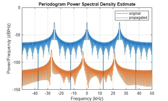
For this wideband signal, you can see that the magnitude of the Doppler shift increases with frequency. In contrast, for narrowband signals, the Doppler shift is assumed constant over the band.

More About

Free-space Time Delay and Path Loss

When the origin and destination are stationary relative to each other, you can write the output signal of a free-space channel as Y(t) = x(t-τ)/L_fsp. The quantity τ is the signal delay and L_fsp is the free-space path loss. The delay τ is given by R/c, where R is the propagation distance and c is the propagation speed. The free-space path loss is given by

$$L_{fsp}=\frac{{(4\pi R)}^2}{{\lambda }^2},$$

where λ is the signal wavelength.

This formula assumes that the target is in the far field of the transmitting element or array. In the near field, the free-space path loss formula is not valid and can result in a loss smaller than one, equivalent to a signal gain. Therefore, the loss is set to unity for range values, R ≤ λ/4π.

When the origin and destination have relative motion, the processing also introduces a Doppler frequency shift. The frequency shift is v/λ for one-way propagation and 2v/λ for two-way propagation. The quantity v is the relative speed of the destination with respect to the origin.

For more details on free space channel propagation, see [2].

Subband Frequency Processing

Subband processing decomposes a wideband signal into multiple subbands and applies narrowband processing to the signal in each subband. The signals for all subbands are summed to form the output signal.

When using wideband frequency System objects or blocks, you specify the number of subbands, N_B, in which to decompose the wideband signal. Subband center frequencies and widths are automatically computed from the total bandwidth and number of subbands. The total frequency band is centered on the carrier or operating frequency, f_c. The overall bandwidth is given by the sample rate, f_s. Frequency subband widths are Δf = f _s/N_B. The center frequencies of the subbands are

$$f_m=\{\begin{array}{c}{f}_c-\frac{f_s}{2}+\left(m-1\right)\Delta f\text{, }{N}_B\text{ even}\\ f_c-\frac{\left(N_B-1\right)f_s}{2N_B}+\left(m-1\right)\Delta f\text{, }{N}_B\text{ odd}\end{array},m=1,\dots ,N_B$$

Some System objects let you obtain the subband center frequencies as output when you run the object. The returned subband frequencies are ordered consistently with the ordering of the discrete Fourier transform. Frequencies above the carrier appear first, followed by frequencies below the carrier.

The phased.WidebandFreeSpace System object uses narrowband time delay and loss algorithms for each subband.

References

[1] Proakis, J. Digital Communications. New York: McGraw-Hill, 2001.

[2] Skolnik, M. Introduction to Radar Systems, 3rd Ed. New York: McGraw-Hill, 2001.

Extended Capabilities

C/C++ Code Generation

Generate C and C++ code using MATLAB® Coder™.

Usage notes and limitations:

See System Objects in MATLAB Code Generation (MATLAB Coder).

Version History

Introduced in R2015b