非線形実行可能性問題の解法、問題ベース

この例では、目的関数を最小化せずに、問題に含まれるすべての制約を満たす点を見つける方法を説明します。

問題の定義

以下の制約について考えてみましょう。

$\begin{array}{l} (y + x^{2})^{2} + 0.1 y^{2} \leq 1 \\ y \leq \exp (- x) - 3 \\ y \leq x - 4 . \end{array}$

すべての制約を満たす点 $(x, y)$ は存在するでしょうか。

問題ベースの解

目的関数のない、制約だけの最適化問題を作成します。

x = optimvar("x");
y = optimvar("y");
prob = optimproblem;
cons1 = (y + x^2)^2 + 0.1*y^2 <= 1;
cons2 = y <= exp(-x) - 3;
cons3 = y <= x - 4;
prob.Constraints.cons1 = cons1;
prob.Constraints.cons2 = cons2;
prob.Constraints.cons3 = cons3;
show(prob)

  OptimizationProblem : 

	Solve for:
       x, y

	minimize :

	subject to cons1:
       ((y + x.^2).^2 + (0.1 .* y.^2)) <= 1

	subject to cons2:
       y <= (exp((-x)) - 3)

	subject to cons3:
       y - x <= -4

最適化変数に対するフィールド x および y をもつ、疑似乱数による開始点の構造体 x0 を作成します。

rng default
x0.x = randn;
x0.y = randn;

x0 から始めて問題を解きます。

[sol,~,exitflag,output] = solve(prob,x0)

Solving problem using fmincon.

Local minimum found that satisfies the constraints.

Optimization completed because the objective function is non-decreasing in 
feasible directions, to within the value of the optimality tolerance,
and constraints are satisfied to within the value of the constraint tolerance.

<stopping criteria details>

sol = struct with fields:
    x: 1.7903
    y: -3.0102

exitflag = 
    OptimalSolution

output = struct with fields:
              iterations: 6
               funcCount: 9
         constrviolation: 0
                stepsize: 0.2906
               algorithm: 'interior-point'
           firstorderopt: 0
            cgiterations: 0
                 message: 'Local minimum found that satisfies the constraints.↵↵Optimization completed because the objective function is non-decreasing in ↵feasible directions, to within the value of the optimality tolerance,↵and constraints are satisfied to within the value of the constraint tolerance.↵↵<stopping criteria details>↵↵Optimization completed: The relative first-order optimality measure, 0.000000e+00,↵is less than options.OptimalityTolerance = 1.000000e-06, and the relative maximum constraint↵violation, 0.000000e+00, is less than options.ConstraintTolerance = 1.000000e-06.'
            bestfeasible: [1×1 struct]
     objectivederivative: 'closed-form'
    constraintderivative: 'forward-AD'
                  solver: 'fmincon'

ソルバーが実行可能点を見つけます。

初期点の重要性

開始する初期点によっては、ソルバーが解を見つけられない場合があります。初期点 x0.x = –1、x0.y = –4 を設定してから、x0 から始めて問題を解きます。

x0.x = -1;
x0.y = -4;
[sol2,~,exitflag2,output2] = solve(prob,x0)

Solving problem using fmincon.

Converged to an infeasible point.

fmincon stopped because it is unable to find a point locally that satisfies
the constraints within the value of the constraint tolerance.

<stopping criteria details>

Consider enabling the interior point method feasibility mode.

sol2 = struct with fields:
    x: -2.1266
    y: -4.6657

exitflag2 = 
    NoFeasiblePointFound

output2 = struct with fields:
              iterations: 144
               funcCount: 318
         constrviolation: 1.4609
                stepsize: 2.9443e-10
               algorithm: 'interior-point'
           firstorderopt: 0
            cgiterations: 300
                 message: 'Converged to an infeasible point.↵↵fmincon stopped because it is unable to find a point locally that satisfies↵the constraints within the value of the constraint tolerance.↵↵<stopping criteria details>↵↵Optimization stopped because the constraint violations are locally stationary ↵but the relative maximum constraint violation, 1.521734e-01, exceeds↵options.ConstraintTolerance = 1.000000e-06.'
            bestfeasible: []
     objectivederivative: 'closed-form'
    constraintderivative: 'forward-AD'
                  solver: 'fmincon'

返された点での実行不可能性を確認します。

inf1 = infeasibility(cons1,sol2)

inf1 = 
1.1974

inf2 = infeasibility(cons2,sol2)

inf2 = 
0

inf3 = infeasibility(cons3,sol2)

inf3 = 
1.4609

cons1 および cons3 は共に解 sol2 で実行不可能です。この結果は、実行可能性問題を調査して解くために複数の開始点を使用することの重要性を強調しています。

制約の可視化

制約を可視化するには、fimplicit を使用して、各制約関数がゼロになる点をプロットします。関数 fimplicit は数値をその関数に渡す一方、関数 evaluate は構造体を必要とします。これらの関数を結合するには、補助関数 evaluateExpr (この例の終わりに掲載) を使用します。この関数は、単に渡された値を適切な名前の構造体に格納します。

メモ: 補助関数 evaluateExpr のコードがスクリプトの最後またはパス上のファイルに必ず含まれるようにしてください。

関数 evaluateExpr がベクトル化された入力に対応していないために発生する警告を回避します。

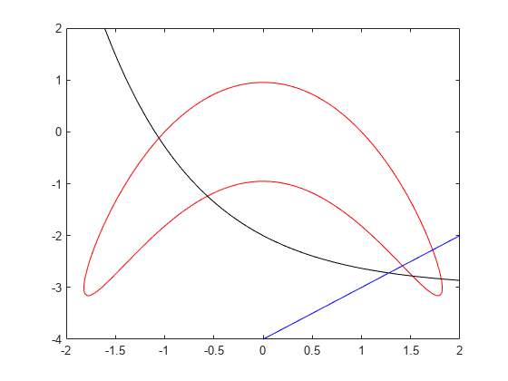
s = warning("off","MATLAB:fplot:NotVectorized");
cc1 = (y + x^2)^2 + 0.1*y^2 - 1;
fimplicit(@(a,b)evaluateExpr(cc1,a,b),[-2 2 -4 2],"r")
hold on
cc2 = y - exp(-x) + 3;
fimplicit(@(a,b)evaluateExpr(cc2,a,b),[-2 2 -4 2],"k")
cc3 = y - x + 4;
fimplicit(@(x,y)evaluateExpr(cc3,x,y),[-2 2 -4 2],"b")
hold off

Figure contains an axes object. The axes object contains 3 objects of type implicitfunctionline.

warning(s);

実行可能領域は、赤線で囲まれた範囲の内側にあり、かつ黒線および青線の下側になります。つまり、実行可能領域は、赤線で囲まれた範囲の右下です。

補助関数

次のコードは、evaluateExpr 補助関数を作成します。

function p = evaluateExpr(expr,x,y)
pt.x = x;
pt.y = y;
p = evaluate(expr,pt);
end

参考

fmincon