プロット関数
最適化実行時のプロット表示
ソルバーの実行中に進捗状況のさまざまな測定をプロットできます。optimoptions の名前と値の引数 PlotFcn を使用して、各反復でソルバーが呼び出すプロット関数を 1 つ以上指定します。関数ハンドル、関数名、または関数ハンドルか関数名の cell 配列を PlotFcn の値として渡します。
各ソルバーではさまざまな定義済みプロット関数を使用できます。詳細については、ソルバーの関数リファレンス ページで PlotFcn オプションの説明を参照してください。
また、カスタムのプロット関数の作成に示すように、カスタムのプロット関数を使用することもできます。出力関数と同じ構造を使用して関数ファイルを記述します。この構造については、出力関数とプロット関数の構文を参照してください。
定義済みプロット関数の使用
この例では、プロット関数を使用して、fmincon "interior-point" アルゴリズムの進行状況を表示する方法を示します。問題は、[最適化] ライブ エディター タスクまたはソルバーを使用した制約付き非線形問題 から取得されます。
勾配を含めて、非線形の目的関数と制約関数を記述します。目的関数は Rosenbrock 関数です。
function [f,g] = rosenbrockwithgrad(x)
% Calculate objective f
f = 100*(x(2) - x(1)^2)^2 + (1-x(1))^2;

if nargout > 1 % gradient required
    g = [-400*(x(2)-x(1)^2)*x(1)-2*(1-x(1));
        200*(x(2)-x(1)^2)];
end
end
制約関数は、解が norm(x)^2 <= 1 を満たすものになります。
function [ineqnonlin,eqnonlin,gradineqnonlin,gradeqnonlin] = unitdisk2(x)
ineqnonlin = x(1)^2 + x(2)^2 - 1;
eqnonlin = [ ];

if nargout > 2
    gradineqnonlin = [2*x(1);2*x(2)];
    gradeqnonlin = [];
end
end
3 つのプロット関数の呼び出しを含む、ソルバーのオプションを作成します。
options = optimoptions(@fmincon,Algorithm="interior-point",...
 SpecifyObjectiveGradient=true,SpecifyConstraintGradient=true,...
 PlotFcn={@optimplotx,@optimplotfval,@optimplotfirstorderopt});
初期点 x0 = [0,0] を作成し、残りの入力を空 ([]) に設定します。
x0 = [0,0];
A = [];
b = [];
Aeq = [];
beq = [];
lb = [];
ub = [];
オプションを含む、fmincon を呼び出します。
fun = @rosenbrockwithgrad;
nonlcon = @unitdisk2;
x = fmincon(fun,x0,A,b,Aeq,beq,lb,ub,nonlcon,options)

Local minimum found that satisfies the constraints.

Optimization completed because the objective function is non-decreasing in
feasible directions, to within the value of the optimality tolerance,
and constraints are satisfied to within the value of the constraint tolerance.

<stopping criteria details>
x = 1×2

    0.7864    0.6177
カスタムのプロット関数の作成
Optimization Toolbox™ ソルバーのカスタムのプロット関数を作成するには、次の構文を使用して関数を記述します。
function stop = plotfun(x,optimValues,state)
stop = false;
switch state
    case "init"
        % Set up plot
    case "iter"
        % Plot points
    case "done"
        % Clean up plots
    % Some solvers also use case "interrupt"
end
end
Global Optimization Toolbox のソルバーでは異なる構文が使用されます。
プロット関数には x、optimValues、および state データが渡されます。構文全体の詳細と optimValues 引数のデータのリストについては、出力関数とプロット関数の構文を参照してください。名前と値の引数 PlotFcn を使用して、ソルバーにプロット関数名を渡します。
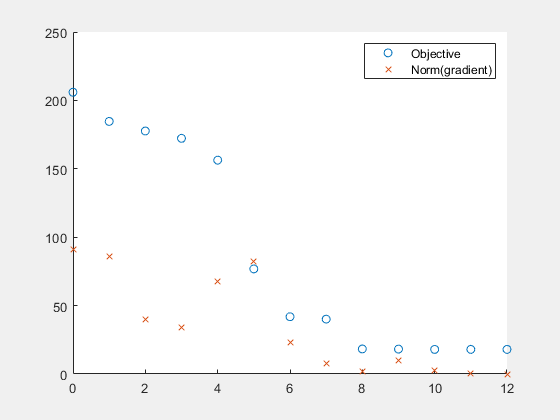
たとえば、この例の最後にリストされている補助関数 plotfandgrad は、スカラー値目的関数の目的関数値と勾配のノルムをプロットします。この例の最後にリストされている補助関数 ras を目的関数として使用します。関数 ras には勾配計算が含まれているので、効率を高めるために、名前と値の引数 SpecifyObjectiveGradient を true に設定します。
fun = @ras;
rng(1) % For reproducibility
x0 = 10*randn(2,1); % Random initial point
opts = optimoptions(@fminunc,SpecifyObjectiveGradient=true,PlotFcn=@plotfandgrad);
[x,fval] = fminunc(fun,x0,opts)
Local minimum found.

Optimization completed because the size of the gradient is less than
the value of the optimality tolerance.

<stopping criteria details>
x = 2×1

    1.9949
    1.9949
fval =
17.9798
プロットは、制約なしの最適化について予期されるとおり、勾配のノルムがゼロに収束することを示しています。
補助関数
次のコードは、plotfandgrad 補助関数を作成します。
function stop = plotfandgrad(x,optimValues,state)
persistent iters fvals grads % Retain these values throughout the optimization
stop = false;

switch state
    case "init"
        iters = [];
        fvals = [];
        grads = [];
    case "iter"
        iters = [iters optimValues.iteration];
        fvals = [fvals optimValues.fval];
        grads = [grads norm(optimValues.gradient)];
        plot(iters,fvals,"o",iters,grads,"x");
        legend("Objective","Norm(gradient)")
    case "done"
end
end
次のコードは、ras 補助関数を作成します。
function [f,g] = ras(x)
f = 20 + x(1)^2 + x(2)^2 - 10*cos(2*pi*x(1) + 2*pi*x(2));
if nargout > 1
    g(2) = 2*x(2) + 20*pi*sin(2*pi*x(1) + 2*pi*x(2));
    g(1) = 2*x(1) + 20*pi*sin(2*pi*x(1) + 2*pi*x(2));
end
end