Control House Heating System Using Nonlinear Model Predictive Control With Neural State-Space Prediction Model

This example shows how to control the thermal dynamics of a house using a nonlinear model predictive controller that uses a neural state-space prediction model.

House Heating System

The house heating system, implemented using Simulink® Simscape™ blocks, contains a heater and a house structure with four parts: inside air, house walls, windows, and roof. The house exchanges heat with the environment through its walls, windows, and roof. Each path is simulated as a combination of thermal convection, thermal conduction, and thermal mass. The house has a temperature sensor.

open_system("house_heating_system");

Control Objectives

The nonlinear model predictive controller (MPC) uses a heater to control house temperature with the following objectives:

• Maintain the temperature within its comfortable zone [20$°$C, 22$°$C]

• Minimize energy cost

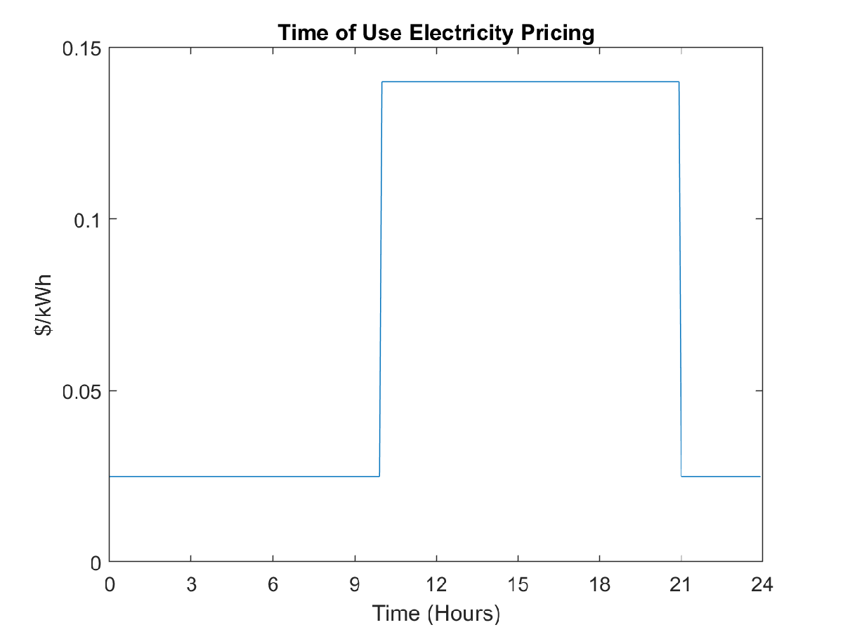
In this example, electricity price flucturates during the day. According to the following figure, the heating cost is most expensive between 10 a.m. and 9 p.m. Therefore you can utilize MPC's preview capability to minimize the electricity cost by keeping the house temperature close to the lower boundary of 20$°$C during on-peak hours.

Nonlinear MPC Using Neural State Space Prediction Model

MPC requires a model to predict future plant behavior. Based on this model, it formulates and solves a constrained optimization problem at each control interval. For this example, assume that you do not have enough domain knowledge to manually derive a low-order, medium-fidelity, first-principle house model that is suitable for MPC to use (or for control system design in general). Therefore use a data-driven approach to identify a dynamic model.

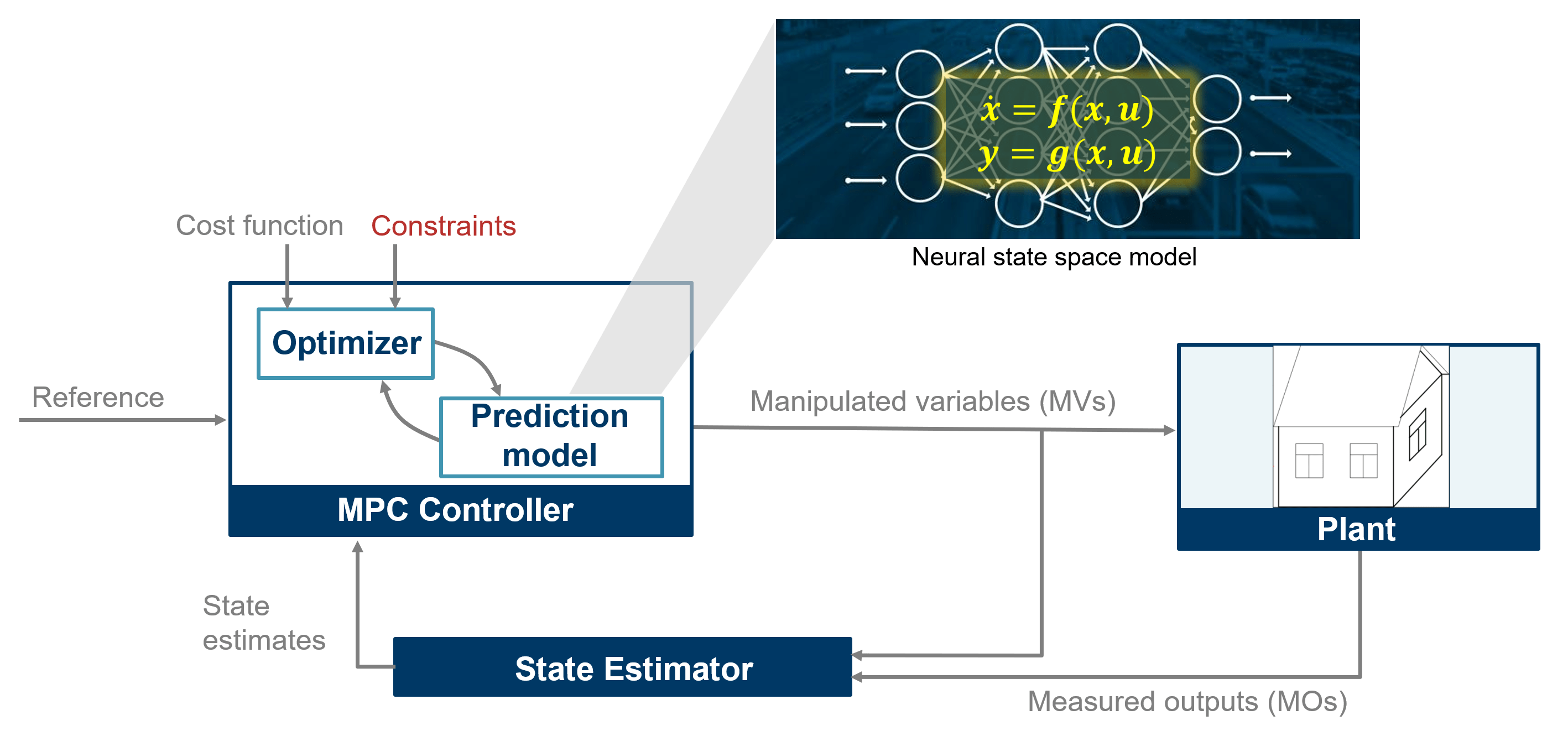
Among several nonlinear modeling techniques available from System Identification Toolbox, neural state space modeling relies on a multi-layer perceptron (MLP) network, which (given enough neurons) can approximate any nonlinear function, including the state transition function required by MPC.

A general MPC control structure is illustrated in the following figure. In this example, state estimation is not used because the state "house temperature" is directly measured.

Prepare Training and Validation Data Sets

To identify a neural state space model, you need state and input trajectories collected from experiments. When these trajectories sufficiently explore the desired state-input space, you can identify a model that provides a good representation of the plant dynamics across the operating range.

Add to the path folders containing the training and validation data and the cost and constraint functions.

addpath(fullfile(pwd,"data"));
addpath(fullfile(pwd,"functions"));

Load the data for neural state space training and validation.

load("training_data.mat");

In this example, the training data set contains 3996 experiments. Each experiment contains one state signal (house temperature) and two input signals (heater input and ambient temperature). The heater input is a manipulated variable, while ambient temperature is a measured disturbance provided to MPC. Each training trajectory contains 72 samples, spaced in intervals of five minutes (300 seconds), for a total experiment duration of six hours. Additionally, a validation data set of one 24-hour long experiment is stored as the last entry in the data set variables X and U.

Train Neural State-Space Prediction Model

To train the model, set do_training to true in the following code block. Since training can take a long time, to load the pre-trained idNeuralStateSpace model nss from a MAT file, leave do_training set to false.

do_training = false;
Ts = 300;
if do_training
    % Fix the random generator seed for reproducible training results.
    rng(0); 
    % Define a discrete-time neural state space model with one state
    % and two inputs, and a sample time of 300 seconds.
    obj = idNeuralStateSpace(1, NumInputs=2, Ts=Ts);
    % Configure the state network to have two hidden layers each with 32
    % nodes.
    obj.StateNetwork = createMLPNetwork(obj, "state", LayerSizes=[32 32]);
    % Create training options object for state network.
    options = nssTrainingOptions("adam");
    % Specify the maximum number of epochs for training to terminate.
    options.MaxEpochs = 300;
    % Divide the data sets into 4 mini-batches, each with 999
    % experiments.
    options.MiniBatchSize = 999;
    % Specify learning rate.
    options.LearnRate = 0.002;
    % Train the state network.
    nss = nlssest(U,X,obj,options,"UseLastExperimentForValidation",true);
else
    load("trained_nss_obj.mat"); 
end

Generate State Function from Neural State-Space Model

The nonlinear MPC controller requires a state transition function defined in a MATLAB® file that returns the time derivative of the system state given the current values of the system state and input. The neural state space model provides a generateMATLABFunction command that generates such a MATLAB function to be used together with MPC. For this example, name this function stateFcn.

generateMATLABFunction(nss,"stateFcn");

Design Multistage Nonlinear MPC Using the State Function

To design a multistage nonlinear MPC, create an nlmpcMultistage object, then set your state function as well as cost and constraint functions at desired stages using dot notation.

Set the prediction horizon to 48 steps (4 hours).

p = (4*3600)/Ts;

Create the multistage nonlinear MPC controller msobj. The first plant input (measured disturbance) is ambient temperature, and the second (measured variable) is the heater input.

msobj = nlmpcMultistage(p,1,'MV',2,'MD',1);

Set the sample time to 300 using dot notation.

msobj.Ts = Ts;

Set the UseMVRate property to true. You can use this option to penalize aggressive control actions.

msobj.UseMVRate = true;

Specify the state name (home temperature), measured variable name, and measured disturbance name.

msobj.States.Name = "T_room"; 
msobj.MV.Name = "P_heat"; 
msobj.MD.Name = "T_atm";

Specify the state function generated from the neural state-space model.

msobj.Model.StateFcn = "stateFcn";

Specify that this function is in discrete-time.

msobj.Model.IsContinuousTime = false;

Specify the cost function for the first and last stages, and specify that each stage has one parameter (the electricity price).

msobj.Stages(1).CostFcn = "myCostFcnwSlackStageFirst";
msobj.Stages(1).ParameterLength = 1;
msobj.Stages(p+1).CostFcn = "myCostFcnwSlackStageLast";
msobj.Stages(p+1).ParameterLength = 1;

Also, specify that the last stage has two slack variables.

msobj.Stages(p+1).SlackVariableLength = 2;

Specify the cost function for the remaining stages. Each has two slack variables and one parameter.

for ct = 2:p
    msobj.Stages(ct).SlackVariableLength = 2;
    msobj.Stages(ct).ParameterLength = 1;
    msobj.Stages(ct).CostFcn = "myCostFcnwSlack";
end

Specify the inequality constraint function, where two slack variables implement the upper and lower temperature bounds as soft constraints.

for ct = 2:p+1
    msobj.Stages(ct).IneqConFcn = "myIneqConFunctionwSlack";
end

Set minimum (0) and maximum (1) bounds for the manipulated variable.

msobj.MV.Min = 0;
msobj.MV.Max = 1;

Generate Jacobian Functions Using Automatic Differentiation

Use generateJacobianFunction to generate, using built-in automatic differentiation, MATLAB functions that return Jacobians of your state, cost, and constraint functions and to add them to your controller.

msobj = generateJacobianFunction(msobj,"state");
msobj = generateJacobianFunction(msobj,"cost");
msobj = generateJacobianFunction(msobj,"ineqcon");

Test the multistage nonlinear MPC controller.

x0 = 20;
u0 = 0;
simdata = getSimulationData(msobj);
simdata.MeasuredDisturbance = 8;
simdata.StageParameter = rand(p+1,1);
validateFcns(msobj,x0,u0,simdata);

Model.StateFcn is OK.
Model.StateJacFcn is OK.
"CostFcn" of the following stages [1 2 3 4 5 6 7 8 9 10 11 12 13 14 15 16 17 18 19 20 21 22 23 24 25 26 27 28 29 30 31 32 33 34 35 36 37 38 39 40 41 42 43 44 45 46 47 48 49] are OK.
"CostJacFcn" of the following stages [1 2 3 4 5 6 7 8 9 10 11 12 13 14 15 16 17 18 19 20 21 22 23 24 25 26 27 28 29 30 31 32 33 34 35 36 37 38 39 40 41 42 43 44 45 46 47 48 49] are OK.
"IneqConFcn" of the following stages [2 3 4 5 6 7 8 9 10 11 12 13 14 15 16 17 18 19 20 21 22 23 24 25 26 27 28 29 30 31 32 33 34 35 36 37 38 39 40 41 42 43 44 45 46 47 48 49] are OK.
"IneqConJacFcn" of the following stages [2 3 4 5 6 7 8 9 10 11 12 13 14 15 16 17 18 19 20 21 22 23 24 25 26 27 28 29 30 31 32 33 34 35 36 37 38 39 40 41 42 43 44 45 46 47 48 49] are OK.
Analysis of user-provided model, cost, and constraint functions complete.

Evaluate MPC Control Performance in Simulink

The house_heating_system Simulink model contains a closed-loop model of the house heating system with the designed MPC controller. Generate price forecast data for the simulation, then use sim to run a 24-hour simulation, and view saved results in the Simulink Data Inspector.

[Tatm_w_for_preview,tou_pricing_for_preview,...
    TinIC,sinePhase,sineAmplitude,sineBias,sineFreq,...
    T_comfort_min,T_comfort_max] = forecastData(Ts);

simout = sim("house_heating_system","StopTime","86400");
open("./SDI_session_with_presaved_simresults.mldatx");

The response shows that before the electricity price jumps at 10 a.m., to save energy, the MPC controller starts to heat the house until the temperature is close to the upper bound.

Remove the previously added folder from the path.

rmpath(fullfile(pwd,"data"));        
rmpath(fullfile(pwd,"functions"));