scaleruler

Add or modify graphic scale on axesm-based map

Syntax

scaleruler

scaleruler on

scaleruler off

scaleruler(Name,Value)

gs = scaleruler(___)

Description

scaleruler toggles the display of the graphic scale on the current axesm-based map. A graphic scale shows distances on the ground at the correct size for the projection. If the map does not have a graphic scale, then scaleruler adds one. If the map has one or more graphic scales, then scaleruler removes them.

scaleruler on adds a graphic scale to the current axesm-based map. You can add multiple graphic scales to the same axesm-based map.

scaleruler off removes all graphic scales from the current axesm-based map.

scaleruler(Name,Value) adds a graphic scale to the current axesm-based map and specifies properties using name-value arguments. For example, "RulerStyle","patches" displays a graphic scale with alternating black and white rectangles.

gs = scaleruler(___) returns the graphic scale. Modify the properties of the graphic scale after you create it by using gs as an input to the setm function.

Examples

Add Graphic Scale to Map

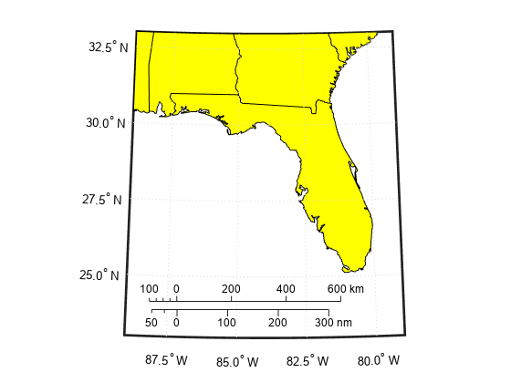
Create a map display of Florida.

usamap("Florida")
geoshow("usastatelo.shp","FaceColor","yellow")

Add a graphic scale. Change the location of the scale by setting the XLoc and YLoc properties. Specify tick locations using the MajorTick property.

gs1 = scaleruler;
setm(gs1,"XLoc",-3.21e5,"YLoc",2.81e6,"MajorTick",0:200:600)

Add a second graphic scale that shows distance in nautical miles. Change the direction of the tick marks and text by setting the TickDir property.

gs2 = scaleruler("Units","nm");
setm(gs2,"XLoc",-3.2e5,"YLoc",2.78e6,"TickDir","down", ...
    "MajorTick",0:100:300,"MinorTick",0:25:50, ...
    "MajorTickLength",km2nm(25),"MinorTickLength",km2nm(12.5))

Customize Appearance of Graphic Scale

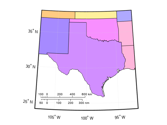
Create a map of Texas and the surrounding states. Your map might look different because the polcmap function randomizes colors.

states = readgeotable("usastatehi.shp");
usamap("Texas")

h = height(states);
faceColors = makesymbolspec("Polygon",{'INDEX',[1 h],'FaceColor',polcmap(h)});

geoshow(states,"DisplayType","polygon","SymbolSpec",faceColors)

Add a graphic scale. By default, the graphic scale displays values in kilometers. Change the location, adjust the major tick marks, and set the font size to 8 points.

scaleruler on
gs1 = handlem("scaleruler1");
setm(gs1,"XLoc",-6.2e5,"YLoc",3.03e6,"MajorTick",0:200:600,"FontSize",8)

Create a second graphic scale using units of nautical miles. Adjust the major and minor tick marks.

scaleruler("Units","nm")
gs2 = handlem("scaleruler2");
setm(gs2,"XLoc",-6.2e5,"YLoc",3.0e6,"MajorTick",0:100:300,"MinorTick",0:25:50, ...
    "TickDir","down","MajorTickLength",km2nm(25),"MinorTickLength",km2nm(12.5),"FontSize",8)

Change the ruler styles.

setm(gs1,"RulerStyle","lines")
setm(gs2,"RulerStyle","patches")

Input Arguments

Name-Value Arguments

Specify optional pairs of arguments as Name1=Value1,...,NameN=ValueN, where Name is the argument name and Value is the corresponding value. Name-value arguments must appear after other arguments, but the order of the pairs does not matter.

Before R2021a, use commas to separate each name and value, and enclose Name in quotes.

Example: scaleruler("Units","nm") creates a graphic scale that displays units in nautical miles

Ticks and Labels

MajorTick — Major tick mark locations

numeric vector

Major tick mark locations, specified as a numeric vector in the units specified by the Units property of the graphic scale.

MajorTickLabel — Major tick mark labels

cell array of character vectors

Major tick mark labels, specified as a cell array of character vectors. The number of character vectors must match the number of major tick locations. By default, the graphic scale uses labels identical to the major tick mark locations.

MajorTickLength — Major tick mark length

numeric scalar

Major tick mark length, specified as a numeric scalar in the units specified by the Units property of the graphic scale.

MinorTick — Minor tick mark locations

numeric vector

Minor tick mark locations, specified as a numeric vector in the units specified by the Units property of the graphic scale.

MinorTickLabel — Minor tick mark labels

cell array of character vectors

Minor tick mark labels, specified as a cell array of character vectors. The number of character vectors must match the number of minor tick locations. By default, the graphic scale uses labels identical to the last minor tick mark location.

MinorTickLength — Minor tick mark length

numeric scalar

Minor tick mark length, specified as a numeric scalar in the units specified by the Units property of the graphic scale.

TickDir — Direction of tick marks and tick labels

"up" (default) | "down"

Direction of tick marks and tick labels, specified as one of these options:

• "up" — Display tick marks and tick labels above the baseline.

• "down" — Display tick marks and tick labels below the baseline.

TickMode — Selection mode for ticks

"auto" (default) | "manual"

Selection mode for ticks, specified as one of these options:

• "auto" — MATLAB^® chooses the ticks. Setting TickMode to "auto" clears any specified ticks and replaces them with default values.

• "manual" — You manually control the ticks. When you specify any tick properties, MATLAB sets TickMode to "manual".

Label — Label

character vector | string scalar

Label that displays along the graphic scale, specified as a character vector or string scalar. You can use the label to indicate the scale of the map, for example "1:50,000,000".

Font

FontName — Font name

supported font name | "FixedWidth"

Font name, specified as a supported font name. To display and print text properly, you must choose a font that your system supports. The default font depends on your operating system and locale.

To use a fixed-width font that looks good in any locale, use "FixedWidth". The fixed-width font relies on the root FixedWidthFontName property. Setting the root FixedWidthFontName property causes an immediate update of the display to use the new font.

FontAngle — Character slant

"normal" (default) | "italic"

Character slant, specified as "normal" or "italic".

FontSize — Font size

9 (default) | positive scalar

Font size, specified as a positive scalar in point units. One point equals 1/72 of an inch. To change the font units, use the FontUnits argument.

FontUnits — Font size units

"points" (default) | "inches" | "centimeters" | "normalized" | "pixels"

Font size units, specified as one of the values in this table.

Units	Description
"points"	Points. One point equals 1/72 of an inch.
"inches"	Inches.
"centimeters"	Centimeters.
"normalized"	Interpret font size as a fraction of the axes plot box height. If you resize the axes, the font size changes accordingly. For example, if the FontSize is 0.1 in normalized units, then the text is 1/10 of the plot box height.
"pixels"	Pixels. Starting in R2015b, distances in pixels are independent of your system resolution on Windows® and Macintosh systems: On Windows systems, a pixel is 1/96 of an inch. On Macintosh systems, a pixel is 1/72 of an inch. On Linux® systems, the size of a pixel is determined by your system resolution.

If you set both the font size and the font units in one function call, you must specify FontUnits first so that the axes correctly interprets the specified font size.

FontWeight — Character thickness

"normal" (default) | "bold"

Character thickness, specified as "normal" or "bold".

MATLAB uses FontWeight to select a font from those available on your system. Not all fonts have a bold weight. Therefore, specifying a bold font weight can still result in the normal font weight.

Position

XLoc — Horizontal location of graphic scale

numeric scalar

Horizontal location of the graphic scale within the axes, specified as a numeric scalar in Cartesian projected coordinates. To view the Cartesian grid labels, use the showaxes function.

You can also interactively move the graphic scale by using your mouse.

YLoc — Vertical location of graphic scale

numeric scalar

Vertical location of the graphic scale within the axes, specified as a numeric scalar in Cartesian projected coordinates. To view the Cartesian grid labels, use the showaxes function.

You can also interactively move the graphic scale by using your mouse.

Color and Styling

Color — Color of graphic scale, tick marks, and text

[0 0 0] (default) | RGB triplet | hexadecimal color code | color name | 'r' | 'g' | 'g' | ...

Color of the graphic scale, tick marks, and text, specified as an RGB triplet, a hexadecimal color code, a color name, or a short name.

For a custom color, specify an RGB triplet or a hexadecimal color code.

• An RGB triplet is a three-element row vector whose elements specify the intensities of the red, green, and blue components of the color. The intensities must be in the range [0,1], for example, [0.4 0.6 0.7].

• A hexadecimal color code is a string scalar or character vector that starts with a hash symbol (#) followed by three or six hexadecimal digits, which can range from 0 to F. The values are not case sensitive. Therefore, the color codes "#FF8800", "#ff8800", "#F80", and "#f80" are equivalent.

Alternatively, you can specify some common colors by name. This table lists the named color options, the equivalent RGB triplets, and hexadecimal color codes.

Color Name	Short Name	RGB Triplet	Hexadecimal Color Code	Appearance
"red"	"r"	[1 0 0]	"#FF0000"
"green"	"g"	[0 1 0]	"#00FF00"
"blue"	"b"	[0 0 1]	"#0000FF"
"cyan"	"c"	[0 1 1]	"#00FFFF"
"magenta"	"m"	[1 0 1]	"#FF00FF"
"yellow"	"y"	[1 1 0]	"#FFFF00"
"black"	"k"	[0 0 0]	"#000000"
"white"	"w"	[1 1 1]	"#FFFFFF"
"none"	Not applicable	Not applicable	Not applicable	No color

Here are the RGB triplets and hexadecimal color codes for the default colors MATLAB uses in many types of plots.

RGB Triplet	Hexadecimal Color Code	Appearance
[0 0.4470 0.7410]	"#0072BD"
[0.8500 0.3250 0.0980]	"#D95319"
[0.9290 0.6940 0.1250]	"#EDB120"
[0.4940 0.1840 0.5560]	"#7E2F8E"
[0.4660 0.6740 0.1880]	"#77AC30"
[0.3010 0.7450 0.9330]	"#4DBEEE"
[0.6350 0.0780 0.1840]	"#A2142F"

RulerStyle — Style of graphic scale

"ruler" (default) | "lines" | ""patches"

Style of the graphic scale, specified as one of these options:

• "ruler" — Resembles the x-axis of an Axes object.

• "lines" — Displays three horizontal lines across the tick marks.

• "patches" — Alternates black and white rectangles in place of lines and tick marks.

LineWidth — Line width

0.5 (default) | numeric scalar

Line width of graphic scale, specified as a numeric scalar in point units.

Scaling

Azimuth — Azimuth of scale computation

0 (default) | numeric scalar

Azimuth of the scale computation, specified as a numeric scalar in the angle units of the current axesm-based map. Within a projection, the scale of a map varies with geographic location and azimuth. This value controls the azimuth along which MATLAB computes the scaling between geographic and projected coordinates.

Lat — Latitude of scale computation

center of displayed map (default) | numeric scalar

Latitude of the scale computation, specified as a numeric scalar in the angle units of the current axesm-based map. Within a projection, the scale of a map varies with geographic location and azimuth. This value controls the latitude along which MATLAB computes the scaling between geographic and projected coordinates.

Long — Longitude of scale computation

center of displayed map (default) | numeric scalar

Longitude of the scale computation, specified as a numeric scalar in the angle units of the current axesm-based map. Within a projection, the scale of a map varies with geographic location and azimuth. This value controls the longitude along which MATLAB computes the scaling between geographic and projected coordinates.

Radius — Name or radius of reference sphere

"earth" (default) | "sun" | "moon" | "mercury" | numeric scalar | ...

Name or radius of reference sphere, specified as "sun", "moon", "mercury", "venus", "earth", "mars", "jupiter", "saturn", "uranus", "neptune", "pluto", or a numeric scalar in units specified by the Units property of the graphic scale. This value controls the scaling between angular and surface distances.

Units — Surface distance units

"kilometer" | "kilometers" | "km" | "degree" | "degrees" | "deg" | ...

Surface distance units, specified as one of these options:

• These angular units.

  Value	Unit Name
  "degree", "degrees", "deg"	Degrees
  "radian", "radians", "rad"	Radians

• Any length unit supported by the validateLengthUnit function.

  Value	Unit Name
  "m", "meter", "meters", "metre", "metres"	Meters
  "cm", "centimeter", "centimeters", "centimetre", "centimetres"	Centimeters
  "mm", "millimeter", "millimeters", "millimetre", "millimetres"	Millimeters
  "micron", "microns"	Microns
  "km", "kilometer", "kilometers", "kilometre", "kilometers"	Kilometers
  "nm", "naut mi", "nautical mile", "nautical miles"	Nautical miles
  "ft", "international ft", "foot", "international foot", "feet", "international feet"	Feet
  "in", "inch", "inches"	Inches
  "yd", "yds", "yard", "yards"	Yards
  "mi", "mile", "miles", "international mile", "international miles"	Miles
  "sf", "survey ft", "US survey ft", "U.S. survey ft", "survey foot", "US survey foot", "U.S. survey foot", "survey feet", "US survey feet", "U.S. survey feet"	U.S. survey feet
  "sm", "survey mile", "survey miles", "statute mile", "statute miles", "US survey mile", "US survey miles", "U.S. survey mile(s)", "U.S. survey miles"	U.S. survey miles (statute miles)
  "Clarke's foot", "Clarkes foot"	Clarke's feet
  "German legal metre", "German legal meter"	German legal metres
  "Indian foot"	Indian feet

This argument is case insensitive.

Output Arguments

gs — Graphic scale

Group object

Graphic scale, returned as a Group object. Modify the properties of a graphic scale by using gs as an input to the setm function. Query the properties of a graphic scale by using gs as an input to the getm function.

Tips

In addition to the syntax scaleruler off, you can remove graphic scales from an axesm-based map by using one of these methods:

• clmo scaleruler — Remove all graphic scales.

• clmo scalerulerN — Remove the Nth graphic scale, such as clmo scaleruler2.

• delete(gs) — Remove the graphic scale specified by gs.

• delete(handlem("scalerulerN")) — Remove the Nth graphic scale, such as delete(handlem("scaleruler2")).

Version History

Introduced before R2006a